Testing mean densities with an application to climate change in Vietnam

1 Introduction

Climate change remains a central focus of scientific inquiry, as its effects on weather patterns, ecosystems, and human livelihoods become increasingly pronounced (Hultgren et al. 2022). According to the World Meteorological Organization, the global mean temperature during the 2011–2020 period has been \(1.10 \pm 0.12^\circ\text C\) higher than the average recorded between 1850 and 1900. Notably, weather-related events accounted for nearly 94% of all recorded disaster-induced displacements over the past decade (World Meteorological Organization 2023). Among the various global climate indicators, near-surface temperature is particularly critical, as it directly influences human well-being and daily activities (Gubler, Fukutome, and Scherrer 2023; World Meteorological Organization 2024; Schlenker and Roberts 2009). Temperatures can be measured using various indicators, such as heat stress, growing degree days, killing degree days, temperature intervals, or the entire temperature distribution (Roberts, Schlenker, and Eyer 2013; Vo, Nguyen, and Simioni 2022; Espagne, Diallo, and Marchand 2019; Schlenker and Roberts 2009; Hultgren et al. 2022). Indeed, considering the entire temperature distribution captures the full range of temperatures throughout each day and over multiple days, offering a more comprehensive and informative perspective (Hsiang et al. 2017; H. T. Trinh, Thomas-Agnan, and Simioni 2023). Vietnam lies closer to the tropics than the equator and is significantly influenced by the East Sea, resulting in a predominantly tropical monsoon climate. The country’s economy is heavily reliant on agriculture, supported by its fertile deltas, mountainous regions, and extensive coastline. Vietnam has been identified as one of the five countries most vulnerable to the impacts of climate change (World Bank Group and Asian Development Bank 2021; Trong-Anh Trinh, Feeny, and Posso 2021). Since 1960, the country’s mean annual temperature has risen by approximately 0.5°C to 0.7°C, with an estimated warming rate of 0.26°C per decade between 1971 and 2010 (World Bank Group and Asian Development Bank 2021). Consequently, as in many other nations, analyzing climate change in Vietnam is of particular interest due to its significant implications for agriculture, especially rice cultivation (Tran and Nguyen 2021; Trong-Anh Trinh, Feeny, and Posso 2021; Trong Anh Trinh 2018).

With the increasing volume of recorded data, data science has seen the rise of new types of observations like functional data. Functional data analysis is currently a very active field of statistics, see (Aneiros et al. 2022). Of particular interest for our application are density-valued data, which can be found in other areas of social sciences (for example age distributions, income distributions, expenditure distributions), and in other fields (for example particle size distributions). Density data require a specific treatment within the framework of functional data analysis, due to their inherent constraints, namely non-negativity and integration to one. It is typically assumed that each observation corresponds to a sampled continuous density function, belonging to an infinite-dimensional function space, as discussed in Petersen, Zhang, and Kokoszka (2022). A smoothing tool is necessary to fill the gap between the discrete data and the continuous temperature density objects and this procedure step is called preprocessing. Among the methods described in Petersen, Zhang, and Kokoszka (2022), we use the Bayes spaces approach first introduced in Egozcue, Díaz–Barrero, and Pawlowsky–Glahn (2006) and later on developed in (Van Den Boogaart, Egozcue, and Pawlowsky-Glahn 2010; Van Den Boogaart, Egozcue, and Pawlowsky-Glahn 2014).

In this paper, we focus on testing mean density functions, investigating their equality to a reference density as well as their equality across groups. Since density functions share similar constraints with compositional vectors, albeit in a continuous form, we build upon techniques from compositional data analysis (CoDA) but also from the functional analysis of variance (FANOVA) framework, introduced in (Ramsay and Silverman 2005; Kokoszka and Reimherr 2017).

Before comparing group means, a first question can be to find whether the expected density is equal to a given reference, for example the uniform density. We adapt the one-sample test from the functional framework (see Zhang 2013) to density functions in Section 3.1.

As outlined by Martín-Fernández, Daunis-i-Estadella, and Mateu-Figueras (2015), the analysis of grouped data typically begins with testing the equality of group means and a widely used approach for this purpose in CoDA is the multivariate analysis of variance (MANOVA) contrast, which needs to be adapted here to continuous objects. On the other hand, the FANOVA techniques (reminded in Section 2.2) must be adapted when applied to density functions because they reside in the constrained space \({B}^2(a,b)\). We present five test statistics in Section 3.2 for the problem of testing the equality of group means of density functions, which we call DANOVA for distributional analysis of variance.

When an ANOVA test leads to a rejection of the null hypothesis of equal group means, a related question of interest is the pairwise comparison of group means (see for example Martín-Fernández, Daunis-i-Estadella, and Mateu-Figueras 2015 who present additional techniques for interpreting the differences between the groups in CoDA). This question is treated in Section 3.3.

Finally, in Section 3.4, to go beyond the global comparisons of densities and do a more local analysis, we adapt a technique based on odds ratios from Maier et al. (2025) to infer the relative mass of the densities over specific intervals.

We apply the above tools to address different questions relative to climate change in Vietnam.

We use the distributions of maximum temperatures in the provinces of Vietnam to compare the six administrative regions in terms of climate change. The dataset and its preprocessing are presented in Section 4. After constructing a trend slope density for each province summarizing its time evolution, we investigate maximum temperature distribution changes through these trend slope densities sample. Then, an analysis of variance of the slope densities in Section 4.5 detects the pairs of regions which differ the most in terms of evolution of the temperature distribution. Finally in Section 4.7, we compare the relative frequencies in different subintervals of the trend distribution allowing a more localized analysis of temperature density evolution.

2 Reminders

2.1 Reminders on functional one-sample problem

In Chapter 5 of Zhang (2013), the functional sample \((f_1, \dots, f_n),\) is assumed to arise from the following model \[f_{i}(x)= f_0(x) + v_{i}(x), \tag{1}\] where \(f_0(x) = {\mathbb E}(f_{i})(x)\) is the unknown mean function and the stochastic error process \(v_{i}\) has mean \(0\).

Two test statistics are available: the \(L^2\)-norm test statistic (Zhang 2013) and the PC approach (Kokoszka and Reimherr 2017).

2.2 Reminders on functional analysis of variance

In the classical framework (Zhang 2013, 144) of functional analysis of variance, or simply FANOVA, we observe \(G\) independent functional samples, denoted by \((f_{g1}, \ldots, f_{gn_g})\) for \(1 \leq g \leq G\), from stochastic processes with values in \(L^2(a,b)\), satisfying for \(1 \leq i \leq n_g\) and \(a \leq x \leq b\) \[f_{gj}(x)= f_g(x) + v_{gj}(x), \tag{2}\] where \(f_g(x) = {\mathbb E}(f_{gj})(x)\) is the unknown mean function in group \(g\) and the stochastic error process \(v_{gj}\) has mean \(0\) and common covariance operator. The total sample size is \(n=\sum_{g=1}^G n_g\). The overall sample mean curve \(\bar f_{..}\) and the group sample mean curves \(\bar f_{g.}\) are respectively defined by \[\begin{aligned} \bar f_{..}(x) &= \frac{1}{n}\sum_{g=1}^G \sum_{i=1}^{n_g} f_{gj}(x) \\ \bar f_{g.}(x) &= \frac{1}{n_g}\sum_{i=1}^{n_g} f_{gj}(x). \end{aligned}\] The pointwise between-group mean square error and the pointwise within-group mean square error at \(x\) are respectively defined by \[\operatorname{SSB}(x) = \sum_{g=1}^G n_g \left( \bar f_{g.}(x) - \bar f_{..}(x) \right)^2 \tag{3}\] and \[\operatorname{SSW}(x) = \sum_{g=1}^G \sum_{i=1}^{n_g} \left( f_{gj}(x)-\bar f_{g.}(x) \right)^2. \tag{4}\] Ramsay and Silverman (2005) extend the classical F-test and propose the pointwise functional F-ratio to test the equality of the group mean curves at a given point \(x\), using the local F-statistic \[F(x)=\frac{\operatorname{SSB}(x)}{\operatorname{SSW}(x)}. \tag{5}\] For a global assessment of the equality of the group mean curves on the whole interval of variation of their argument, Zhang and Chen (2007) and Zhang (2013) introduce \(L^2\)-norm based tests as well as F-type test statistics. Later on, Zhang and Liang (2014) propose the GPF test based on the integral of the pointwise F-ratio statistic (see Section 3.2) and the \(F_\text{max}\) test based on the maximum of the pointwise F-test. It is then necessary to approximate the null distribution of these statistics. This can be achieved using a permutation based procedure as in Ramsay and Silverman (2005) or a bootstrap procedure as in Zhang et al. (2019).

2.3 Reminders on distributional data analysis and Bayes spaces

Egozcue, Díaz–Barrero, and Pawlowsky–Glahn (2006) and Van Den Boogaart, Egozcue, and Pawlowsky-Glahn (2010; 2014) define the Bayes spaces of probability density functions relative to a reference measure \(\lambda\) on an interval of \(\mathbb R\), in a similar fashion as \(L^2(\lambda)\) spaces. In the following, the measure \(\lambda\) will be the Lebesgue measure on a finite interval \([a,b]\) and we will denote these spaces by \({B}^2(a,b)\). We consider the separable Hilbert space \(L^2_0(a,b)\) of square-integrable functions with a zero integral on \((a,b)\) equipped with the inner product \(\langle f,g \rangle_{L^2} = \int_a^b fg \,\mathrm d\lambda\). For any measurable function \(\varphi : [a,b] \rightarrow \mathbb R\) that is positive almost everywhere and such that the function \(\log (\varphi)\) is integrable, we can define its centered log-ratio transform \(\operatorname{clr}(\varphi)\) \[ x \in [a,b] \mapsto \log(\varphi (x)) - \frac1{b-a} \int_a^b \log(\varphi)(u) \mathrm du. \tag{6}\] Note that by construction \(\operatorname{clr} (\varphi) \in L^2_0(a,b).\) Conversely for each \(f \in L^2_0 (\lambda)\), the equivalence class \(\operatorname{clr}^{-1} (f) = \{ \alpha \exp (f), \alpha >0 \}\) contains positive functions that are equal almost everywhere, up to a multiplicative constant. Among them there is a unique probability density function \(\varphi\) (thus satisfying \(\int_a^b \varphi(u) \, \mathrm du = 1\)) that we use to represent \(\operatorname{clr}^{-1} (f)\). For any element \(p\) of \(\operatorname{clr}^{-1} (f),\) the closure of \(p,\) denoted by \({\cal C}(p)\), is defined to be \(\varphi\).

Then the Bayes Hilbert space with Lebesgue reference measure on the interval \([a,b]\) is the set of probability density functions \[{B}^2 (a,b) = \left\{ \operatorname{clr}^{-1} (f), f \in L^2_0 (a,b) \right\}\] equipped with the only separable Hilbert space structure \((\oplus, \odot, \langle \cdot, \cdot \rangle_{B^2})\) that makes the centered log-ratio transform an isometry between \(({B}^2 (a,b), \oplus, \odot, \langle \cdot, \cdot \rangle_{{B}^2})\) and \((L^2_0 (a,b), +, \cdot, \langle \cdot, \cdot \rangle_{L^2})\). The resulting addition \(\oplus\) is called Aitchison perturbation (\(\ominus\) denoting the negative perturbation) and the scalar multiplication \(\odot\) is called Aitchison powering.

Since it is important to understand some further developments, we recall that, given two elements \(\varphi_1\) and \(\varphi_2\) of the Bayes space, the perturbation density \(\varphi_2 (x) \ominus \varphi_1 (x)\) is the closure of the ratio \(\frac{\varphi_2 (x)}{\varphi_1 (x)}\), which is equal to \(\frac{{\varphi_2 (x)}/{\varphi_1 (x)}}{\int_a^b {\varphi_2 (u)}/{\varphi_1 (u)}du}\).

Following Van Den Boogaart, Egozcue, and Pawlowsky-Glahn (2014), it is also possible to use the centered log-ratio transform in order to transport the Borel sets to \({B}^2 (a,b)\), as well as the expectation and covariance of \(L^2_0 (a,b)\)-valued random variables. For a random density \(\varphi\) in \({B}^2(a,b)\), one can define the expected value in the Bayes space as: \[ \mathbb{E}^B(\varphi) = \operatorname{clr}^{-1} (\mathbb E [\operatorname{clr}(\varphi)]) \tag{7}\] and the covariance operator, for \(\psi \in B^2(a,b)\), by: \[\begin{split} \operatorname{Cov}^B [\varphi] (\psi) &= \operatorname{clr}^{-1} (\operatorname{Cov} [\operatorname{clr} \varphi] (\operatorname{clr} \psi)) \\ &= \mathbb{E}^B \left[ \langle\varphi \ominus \mathbb E ^B (\varphi), \psi \rangle_{B^2} \odot \left( \varphi \ominus \mathbb E^B (\varphi) \right) \right]. \end{split} \tag{8}\]

3 Testing and interpreting mean densities in the Bayes space

All testing procedures in this section involve hypotheses about the global behavior of mean densities in the whole interval \([a,b].\) In the application, the global tests of this section will be applied to the samples of trend slope densities in order to investigate the regional effect on climate change.

3.1 One-sample problem

In this section, we consider a sample of densities \(\varphi_i, i=1, \ldots n\) in the Bayes space \(B^2(a,b)\) distributed as \(\varphi\). We are given a reference density \(\varphi_0\) of particular interest and we wish to test the equality to \(\varphi_0\) of the mean density \(\mathbb{E}^B(\varphi)\): \[H_0: {\mathbb E}^B (\varphi) = \varphi_0.\] Since \[\begin{split} {\mathbb E}^B (\varphi) = \varphi_0 &\Leftrightarrow \operatorname{clr} {\mathbb E}^B (\varphi) = \operatorname{clr} \varphi_0 \\ &\Leftrightarrow {\mathbb E} (\operatorname{clr} \varphi) = \operatorname{clr} \varphi_0, \end{split}\] the global one-sample test on mean densities is equivalent to a one sample test in the \(L^2(a,b)\) space on the clr transformed densities \(f_i = \operatorname{clr} (\varphi_i)\) for which we may apply a classical one sample test for functional data as described in Chapter 5 of Zhang (2013). As in Zhang (2013), the functional sample \((f_1, \dots, f_n),\) is assumed to arise from model Equation 1.

Two test statistics are available: the \(L^2\)-norm test statistic (Zhang 2013) and the PC approach (Kokoszka and Reimherr 2017). We now adapt them to our density framework.

\(L^2\)-norm approach

We consider the following statistic defined in the Bayes space by \[\begin{split} T_\text{norm} &= n \| \bar{\varphi}_{.} - \varphi_0 \|^2_{B^2(a,b)} \\ &= n \| \operatorname{clr} (\bar{\varphi}_{.}) - \operatorname{clr} (\varphi_0) \|^2_{L^2_0(a,b)}, \end{split}\] where \(\bar{\varphi}_{.}\) denotes the sample mean of the densities in \(B^2(a,b)\). We can see that it does correspond to an \(L^2\)-norm statistic to test the equality in \(L^2_0\) of the clr transform \(f_i= \operatorname{clr} (\varphi_i)\) of our sample of densities \(\varphi_i\). We can therefore apply the classical one sample test for functional data described in Chapter 5 of Zhang (2013).

The asymptotic distribution of this statistic under the null is that of a linear combination of chi-squared statistics weighted by the eigenvalues of the covariance operator, see (Kokoszka and Reimherr 2017). For the computation of the \(p\)-value of the test, the eigenvalues have to be estimated using FPCA and Kokoszka and Reimherr (2017) provide code for the computation of the \(L^2\)-norm.

PC approach

To eliminate the dependence of the limiting distribution upon the unknown eigenvalues, Kokoszka and Reimherr (2017) propose to truncate the Functional Principal Component Analysis (FPCA) and use a Hotelling-type test statistic. It turns out that this statistic applied to the clr-transformed densities coincides with that obtained with the simplicial FPCA in \(B^2(a,b)\) from Hron et al. (2016). Keeping the first \(p\) terms, the statistic \(T_{\operatorname{PC}}\) is given by \[\begin{split} T_{\operatorname{PC}} &= n\sum_{k=1}^p \frac{\langle \operatorname{clr} (\bar{\varphi}_{.}) - \operatorname{clr} (\varphi_0), \hat{v}_k \rangle_{L^2_0(a,b)}^2}{\hat \lambda_k} \\ &= n\sum_{k=1}^p \frac{\langle \bar{\varphi}_{.} \ominus \varphi_0, \operatorname{clr}^{-1}(\hat{v}_k) \rangle_{B^2(a,b)}^2}{\hat \lambda_k}. \end{split}\] where \(\hat\lambda_k\) are the estimated non-null eigenvalues and \(\hat v_k\) the corresponding estimated eigenfunctions in \(L^2_0(a,b)\) from the FPCA. The limiting distribution of \(T_{\operatorname{PC}}\) under the null is then a simple chi-squared with \(p\) degrees of freedom. Kokoszka and Reimherr (2017) recommend using the smallest value of \(p\) for which the explained variance exceeds \(85 \%\), and to use the norm approach otherwise.

3.2 Distributional ANOVA

We observe \(G\) independent samples of densities, denoted by \((\varphi_{g1}, \ldots, \varphi_{gn_g})\) for \(1 \leq g \leq G\), from stochastic processes with values in \(B^2(a,b)\), satisfying for \(1 \leq i \leq n_g\) and \(a \leq x \leq b\) \[\varphi_{gj}(x)= (\varphi_g \oplus u_{gj})(x), \tag{9}\] where \(\varphi_g(x) = {\mathbb E}^B(\varphi_{gj})(x)\) is the unknown mean density in group \(g\) and the stochastic error process \(u_{gj}\) has mean equal to the uniform distribution on \((a,b)\) and common covariance operator (defined by Equation 8 in Bayes spaces). The total sample size is \(n=\sum_{g=1}^G n_g\). As above the overall sample mean density is defined as \[\bar \varphi_{..} (x) = \frac1n \odot \bigoplus_{g=1}^G \bigoplus_{i=1}^{n_g} \varphi_{gj} (x)\] and the sample mean density in group \(g\) as \[\bar\varphi_{g.} (x) = \frac1{n_g} \odot \bigoplus_{i=1}^{n_g} \varphi_{gj} (x).\] Applying the FANOVA formulas to the clr-transformed densities, we adapt the FANOVA framework to densities and define the pointwise between-group mean square error and the pointwise within-group mean square error at \(x\) by \[\operatorname{SSB}(x) = \sum_{g=1}^G {n_g} (\operatorname{clr}(\bar\varphi_{g.})(x) - \operatorname{clr}(\bar\varphi_{..})(x))^2 \tag{10}\] and \[\operatorname{SSW}(x) = \sum_{g=1}^G \sum_{i=1}^{n_g} (\operatorname{clr}(\varphi_{gj})(x) - \operatorname{clr}(\bar\varphi_{g.}) (x))^2 \tag{11}\]

Using the notations of Section 2.3, the objective of DANOVA is to test the null hypothesis \(H_0\) that the \(G\) group mean densities \({\mathbb E}^B(\varphi_g)\) are equal against the usual alternative that at least two means are different, where mean density here is understood in the Bayes space sense: \[H_0: \forall g, \quad {\mathbb E}^B (\varphi_{gj}) = {\mathbb E}^B (\varphi_{1j}). \tag{12}\] Let us first note that for two densities \(\varphi_1\) and \(\varphi_2\) we have the following equivalence \[{\mathbb E}^B (\varphi_1) = {\mathbb E}^B (\varphi_{2}) \Leftrightarrow {\mathbb E} (\operatorname{clr }\varphi_{1}) = {\mathbb E} (\operatorname{clr }\varphi_{2}), \tag{13}\] since the clr of the expected density in the Bayes sense is equal to the expected value in the classical sense of the clr of the density in the corresponding \(L^2_0\) space. Therefore, the assumption Equation 12 is equivalent to \[H_0: \forall g, \quad {\mathbb E} (\operatorname{clr}\varphi_{gj}) = {\mathbb E} (\operatorname{clr}\varphi_{1j}).\] In order to adapt FANOVA to DANOVA, we can thus simply apply the FANOVA techniques to the clr transformed densities in the functional space \(L^2_0.\) The R package fdANOVA (described in Górecki and Smaga 2019) provides several FANOVA options and we focus on the following five test statistics. Their evaluation requires the computation of the following quantities: the pointwise variations \(\operatorname{SSB}(x)\) and \(\operatorname{SSW}(x)\) from Equation 10 and Equation 11, and pairwise negative perturbations between group means for the statistic proposed by Cuevas, Febrero, and Fraiman (2004). Let us briefly describe the five test statistics and try to provide when possible a Bayes space expression.

\(\operatorname{L^2B}\) statistic

We adapt the \(L^2\)-norm based test statistic given in the framework of FANOVA (Zhang and Chen 2007) to the context of densities: \[\operatorname{L^2B} = \int_a^b \operatorname{SSB}(x)dx, \tag{14}\] where \(\operatorname{SSB}(x)\) is given by Equation 10. Note that an alternative formula for \(\operatorname{L^2B}\) can be written using the norm of the Bayes space: \[\operatorname{L^2B} = \sum_{g=1}^G n_g \| \bar\varphi_{g.} \ominus \bar\varphi_{..}\|^2_{B^2}, \tag{15}\] which shows that this statistic is invariant under almost-everywhere equality. In the Górecki and Smaga (2019) fdANOVA R package, the L2B implementation uses an asymptotic distribution of the test statistic.

\(\operatorname{FB}\) statistic

The F-type tests from Shen and Faraway (2004) and Zhang (2011) use both within and between variation: \[\begin{split} \operatorname{FB} &= \frac{{\int_a^b \operatorname{SSB}(x)dx}/(G-1)}{\int_a^b \operatorname{SSW}(x)dx /(n-G)} \\ &= \frac{\sum_{g=1}^G n_g \| \bar\varphi_{g.} \ominus \bar\varphi_{..}\|^2_{B^2}/(G-1)}{\sum_{g=1}^G \sum_{i=1}^{n_g} \| \varphi_{gj} \ominus \bar\varphi_{g.}\|^2_{B^2}/(n-G)}. \end{split} \tag{16}\] We choose the bias-reduced FB implementation for the computation of the \(p\)-value. Under the null hypothesis, this statistic is asymptotically equal to a linear combination of independent \(\chi^2\) for the numerator and the denominator, and can thus be approximated by a Fisher distribution (Zhang 2011, Theorem 1 and equation (2.16)). The test statistic coincides with that of Van Den Boogaart, Egozcue, and Pawlowsky-Glahn (2014) by the second equality in Equation 16. However, Van Den Boogaart, Egozcue, and Pawlowsky-Glahn (2014) use a bootstrap procedure rather than the above approximation.

\(\operatorname{CS}\) statistic

The CS statistic from Cuevas, Febrero, and Fraiman (2004) uses pairwise differences. When applied to clr of densities, due to the linearity of \(\operatorname{clr}\), we get \[\begin{split} \operatorname{CS} &= \sum_{g<g'} n_g \int_a^b \left( \operatorname{clr} {\bar\varphi_{g.}}(x)- \operatorname{clr} {\bar\varphi_{g'.}}(x) \right)^2dx \\ &= \sum_{g<g'} n_g \| \bar\varphi_{g.} \ominus \bar\varphi_{g'.} \|^2_{B^2}. \end{split} \tag{17}\] The CS implementation in the fdANOVA package uses a heteroscedastic assumption and parametric bootstrap. Note that an alternative formula for CS is the sum of the Bayes norms of all pairwise differences between groups.

\(\operatorname{GPF}\) statistic

The GPF statistic from Zhang and Liang (2014) integrates the pointwise F-ratio instead of integrating separately the pointwise within and between variations: \[\operatorname{GPF} = \int_a^b \frac{\operatorname{SSB}(x)/(G-1)}{\operatorname{SSW}(x)/(n-G)}dx. \tag{18}\] Under the null hypothesis, this statistic is asymptotically equal to a linear combination of independent \(\chi^2\), which can be approximated by a \(\chi^2\)-distribution (Zhang and Liang 2014, Proposition 1). In the implementation of the fdANOVA package, GPF is divided by \(b-a\), and the null distribution is modified accordingly. Górecki and Smaga (2018) (page 5) claim that the GPF test is more powerful than the F-type tests.

\(F_{\max}\) statistic

The \(F_{\max}\) statistic from Zhang et al. (2019) rather computes the supremum of the pointwise F-ratio instead of integrating it as in GPF: \[F_{\max} = \sup_{x \in (a,b)} \frac{\operatorname{SSB}(x)/(G-1)}{\operatorname{SSW}(x)/(n-G)}. \tag{19}\] We consider the implementation Fmaxb which bootstraps the distribution under the null hypothesis. The statistic \(F_{\max}\) is the only one that is not invariant under almost-everywhere equality: changing one value of a density in the dataset might change the value of \(F_{\max}\).

Finally, note that the statistics GPF and \(F_{\max}\) cannot be written straightforwardly in terms of norms in the Bayes space. Górecki and Smaga (2018) compute empirical powers of some FANOVA tests and conclude that there is no method that performs best in all situations.

3.3 Pairwise comparisons

When the test of equality of group mean densities is significant, conducting a post-hoc analysis of pairwise group mean comparisons can help identify which pairs differ. The null hypothesis for comparing groups \(g\) and \(g'\) is: \[H_0: \quad {\mathbb E}^B (\varphi_{gj}) = {\mathbb E}^B (\varphi_{g'j}),\] which is equivalent to \[H_0: \quad {\mathbb E} (\operatorname{clr}\varphi_{gj}) = {\mathbb E} (\operatorname{clr}\varphi_{g'j}).\]

Testing whether the mean density in group \(g_1\) is equal to the mean density in group \(g_2\) can be viewed as a two-sample ANOVA test. A multiple testing correction is necessary when performing these tests for all pairs of groups.

3.4 Interval-wise interpretation

The global tests presented in the previous section, whether one-sample tests or analysis of variance, enable us to draw inferences about differences in the behavior of mean densities across the entire range of the underlying random variable. Now, we aim to make more localized statements regarding specific intervals of this range.

Unfortunately, the idea of adapting local tests from FANOVA does not work for two reasons. First of all, the meaning of a test of the equality of two mean densities evaluated at a given point \(x\) is unclear since densities are only defined almost everywhere, unless we impose continuity restrictions. The second reason is that the equivalence Equation 13 between the equality of two mean densities in a Bayes space and the equality of their clr transform is not valid anymore at the local level because the clr transform evaluated at \(x\) involves all values of the log density and not only its value at \(x\).

For these reasons, we now turn attention to some interpretation tools presented in Maier et al. (2024) based on odds ratios.

For some subintervals \(I \subset [a,b]\) we wish to compare the relative probability to be in \(I\) versus its complement in \((a,b)\) between two densities \(\varphi_1\) and \(\varphi_2\). Let us start with an infinitesimal comparison that only implies any two points \(x,z\) in \((a,b)\).

Given \(\varphi_1\) and \(\varphi_2\), Maier et al. (2024, 10 and 11, Proposition 3.1) define the infinitesimal odds ratios \(\operatorname{OR}_{x\mid z}\) of \(\varphi_2\) versus \(\varphi_1\) as \[\operatorname{OR}_{x\mid z} = \frac{\frac{{\varphi}_2(x)}{{ \varphi}_2(z)}}{\frac{{\varphi}_1(x)}{{ \varphi}_1 (z)}}. \tag{20}\] \(\operatorname{OR}_{x\mid z}\) is the ratio of the odds of \(x\) versus \(z\) for \(\varphi_2\) by the odds of \(x\) versus \(z\) for \(\varphi_1\). Let us prove that this quantity coincides with the relative density of the negative perturbation \(\beta = \varphi_2 \ominus \varphi_1\) at the two points \(x\) and \(z\) in \((a,b)\). Indeed, we can first rewrite the double ratio differently with \(x\) in the top ratio and \(z\) in the bottom one and then use the fact that the integral of the numerator is the same as that of the denominator: \[\begin{split} \operatorname{OR}_{x\mid z} &= \frac{\frac{\varphi_2(x)}{\varphi_1(x)}}{ \frac{\varphi_2(z)}{ \varphi_1 (z)}} = \frac{{\cal C}(\frac{\varphi_2(x)}{\varphi_1(x)})}{{\cal C}(\frac{\varphi_2(z)}{\varphi_1(z)})} \\ &= \frac{{\varphi}_2(x) \ominus { \varphi}_1(x)}{{ \varphi}_2(z) \ominus{ \varphi}_1(z)} = \frac{\beta (x)}{\beta (z)}. \end{split} \tag{21}\] where \(\cal C\) denotes the closure operator whose definition is recalled in Section 2.3. This justifies that we write the infinitesimal odds ratios between two densities \(\varphi_1\) and \(\varphi_2\) as a function \(\operatorname{OR}_{x\mid z} (\beta)\) of their negative perturbation \(\beta\).

Let us now use these infinitesimal odds ratios to compare the densities on subintervals of \([a,b]\). Using part (a) of Proposition 3.1 in Maier et al. (2024), which states that if \(\operatorname{OR}_{x\mid z} (\beta) > 1\) for all \(x,z\) when \(x\) is in a given interval \(A\) and \(z\) in a given interval \(B\), we may conclude that conditional on the underlying variable being in \(A\) or \(B\), the odds (according to the density \({\varphi}_2\)) of being in \(A\) are larger than the odds (according to the density \({\varphi}_1\)) of being in \(A\). Because the probability of an event is an increasing function of its odds, the same is true for the corresponding probabilities so that going from \(\varphi_1\) to \(\varphi_2\) there is a transfer of the probability mass from \(B\) to \(A\).

Using the fact that \(\operatorname{OR}_{x\mid z} (\beta) >1\) is equivalent to \(\beta(x) > \beta(z)\), we are going to show that the curve of \(\beta\) allows to draw conclusions about the relative size of the probability mass of some chosen intervals according to \(\varphi_1\) and \(\varphi_2\). For a given level \(\tau = \beta(x_0) >0\), let the collection of intervals (or unions of intervals) \(A_{\tau}\) be defined by \(A_{\tau} = \{ x: \beta(x) > \tau \}\) and let \(A_{\tau}^c\) be its complement. Then we have for almost all \(x \in A_{\tau}\) and almost all \(z \in A_{\tau}^c\) \[\operatorname{OR}_{x\mid z}(\beta) = \frac{\beta(x)}{\beta(x_0)}\frac{\beta(x_0)}{\beta(z)} > 1. \tag{22}\] Therefore, we may say that the probability to lie in \(A_{\tau}\) under the distribution of \(\varphi_2\) is higher than that according to the distribution of \(\varphi_1\).

As we can see in Equation 21 this type of interpretation is useful as soon as we are interested in a negative perturbation between two densities. In particular, as we will see in the next section, we can use it to compare in a local fashion two mean temperature densities in two regions or at two different dates. It will also be useful to interpret regional trends in temperature distributions which turn out to be negative perturbations between the temperature density at two consecutive times. More generally, provided we have a linear model for our density objects, the same tool can be used to make marginal effects interpretations for a scalar covariate parameter.

4 Trends in yearly temperature distributions in Vietnam over the period 1987-2016

4.1 Description

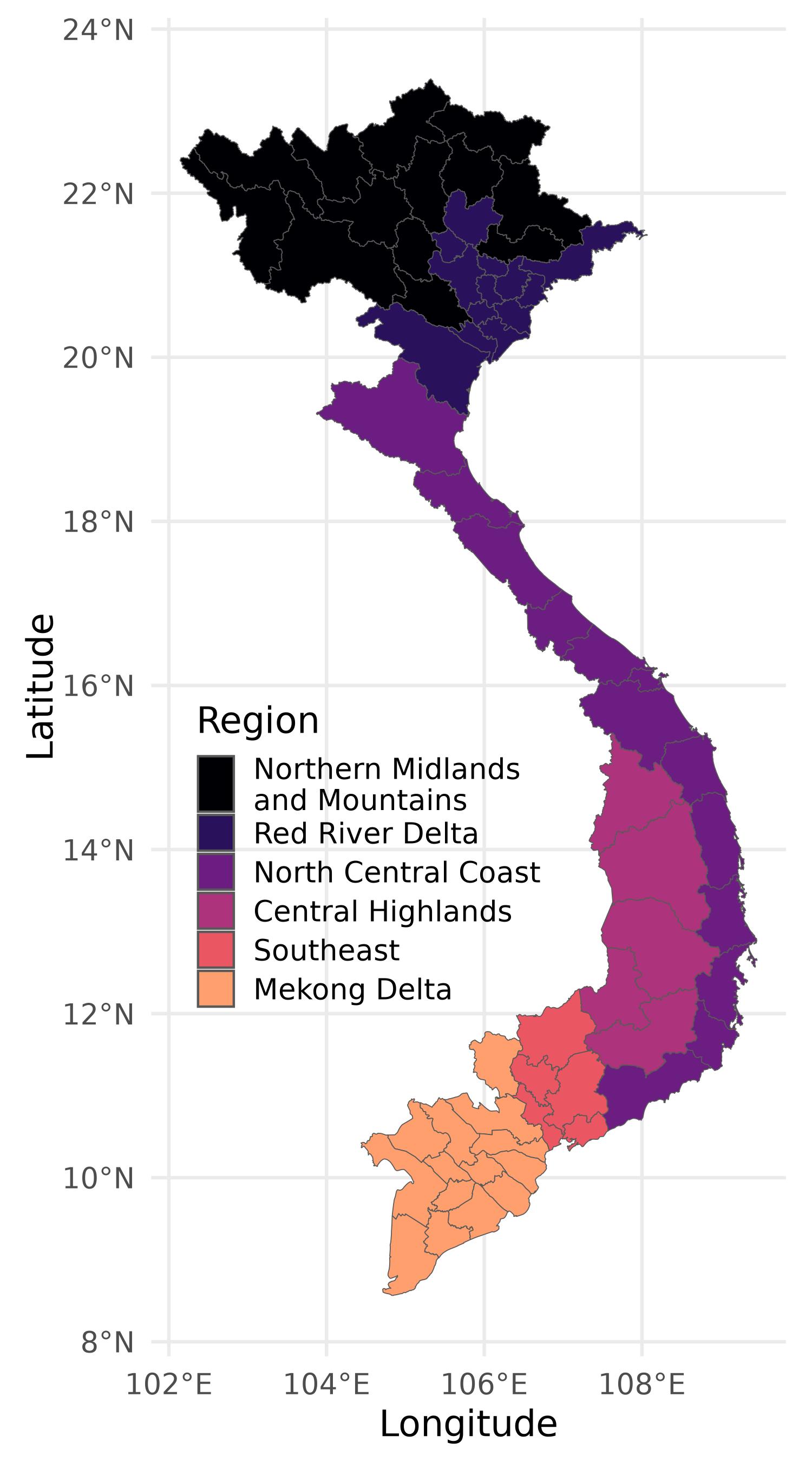
The climate data used in this study comprises daily temperatures and precipitation, sourced from the Climate Prediction Center (CPC) database, developed by the National Oceanic and Atmospheric Administration (NOAA). This data provides historical records of the maximum and minimum temperatures for a 0.5-degree by 0.5-degree grid of latitude and longitude. For this study, we focus exclusively on maximum temperatures as they are a direct indicator of heat stress on both humans and the environment. The data spans the years 1987 to 2016. In order to address the discrepancy between the geographical coordinates and the municipalities of Vietnam (63 provinces), Espagne, Diallo, and Marchand (2019) performed a spatial interpolation step from the gridded data to the provincial level.

This process results in 365 or 366 daily maximum temperature records for each province and year.

During the study period, maximum temperatures (hereafter denoted \(T_\text{max}\)) range from -5°C to nearly 45°C. However, extreme cold and extreme heat are rare. Moreover subintervals with no observations result in zero density value which is problematic for the logarithm. For the purpose of our analysis, we focus on a temperature range of 12°C to 40°C. Temperatures below 12°C are adjusted upward to 12°C, while temperatures exceeding 40°C are capped at 40°C. As we can see on Figure 1, there are \(n=63\) provinces in Vietnam grouped into \(G=6\) socioeconomic regions. We use the following acronyms for the regions: NMM for Northern Midlands and Mountains region (\(n_1=14\) provinces), RRD for Red River Delta region (\(n_2=12\) provinces), NCC for North Central Coast region (\(n_3=13\) provinces), CHR for Central Highlands region (\(n_4=5\) provinces), SR for Southeast region (\(n_5=6\) provinces) and MDR for Mekong Delta region (\(n_6=13\) provinces). Trong-Anh Trinh, Feeny, and Posso (2021) highlight the fact that the regions have their own weather peculiarities. Some regions in the north have four seasons: winter, spring, summer, and autumn, while some regions in the south experience two distinct seasons: the dry season (November to April) and the rainy season (May to October) (Trong-Anh Trinh, Feeny, and Posso 2021; World Bank Group and Asian Development Bank 2021). For example, according to Trong-Anh Trinh, Feeny, and Posso (2021), during the period 1960-2000 winter temperatures rose faster than those of the summer, and temperatures in the northern zones rose faster than in the southern zones. The objective of this application is first of all to determine whether there is a regional factor in the evolution of temperature distributions over time. The groups are thus the six regions of Vietnam. Secondly, we will describe the changes in regional temperature distributions in some subintervals of the temperature range.

Figure 1: Map of the provinces of Vietnam colored by region.

Source: Article Notebook

4.2 Smoothing

We will assume that the observed data arise from random densities, themselves sampled from a hypothesized and unknown distribution on a Bayes space. Since the elements of the Bayes spaces are density functions, whereas the observed data (usually samples of real-valued observations or histograms) is always discrete, a preprocessing step is necessary to transform the observed samples or histograms into a sample of probability density functions. We will follow the preprocessing procedure of (J. Machalová, Hron, and Monti 2016; Jitka Machalová et al. 2021) to transform our yearly samples of maximum temperatures at the province level into density functions that we assume to belong to a finite-dimensional subspace \(\mathcal C_q^\Delta (a,b)\) of the Bayes Hilbert space \(B^2(a,b)\), made of compositional splines. A compositional spline (CB-spline) is a probability density function whose logarithm is a polynomial spline.

The process starts by the choice of a basis of normalized B-spline functions for the space \(\mathcal S_d^\Delta (a,b) \subset L^2(a,b),\) of polynomial splines of order \(d\) (degree less than or equal to \(d-1\)) and inside knots \(\Delta = (\delta_1, \ldots, \delta_k)\), of dimension \(d+k\) (see Schumaker 1981 for a complete description). To accommodate the zero-integral constraint, J. Machalová, Hron, and Monti (2016) introduce the ZB-spline functions, denoted by \(Z_\ell(x), 1 \leq \ell \leq d+k-1\) for the subspace \(\mathcal Z_d^\Delta (a,b) = \mathcal S_d^\Delta (a,b) \cap L^2_0(a,b)\) of dimension \(d+k-1\), the loss of one dimension being due to the zero-integral constraint. Finally the inverse clr of the ZB-spline basis functions, called the CB-spline basis functions, denoted by \(C_\ell =\operatorname{clr}^{-1}(Z_\ell)\) generate the space \(\mathcal C_d^\Delta (a,b),\) a Euclidean subspace of \({B}^2 (a,b)\) of dimension \(k+d-1,\) made of compositional splines on \([a,b]\) of order \(d\) with knots sequence \(\Delta.\) The expansion Equation 23 of a density \(\pi_{gj}^{t}\) of the subspace \(\mathcal C_d^\Delta (a,b)\) of \({B}^2(a,b)\) and the corresponding expansion Equation 24 of its clr transform in the corresponding ZB-spline basis generating the space \(\mathcal Z_d^\Delta (a,b)\) are then given by: \[\pi_{gj}^{t}(x) = \bigoplus_{\ell=1}^{d+k-1} \left[\pi_{gj}^{t}\right]^{C_\ell}\odot C_\ell(x) \tag{23}\] or equivalently \[\operatorname{clr}(\pi_{gj}^{t})(x) = \sum_{\ell=1}^{d+k-1} \left[\pi_{gj}^{t}\right]^{C_\ell} Z_\ell(x), \tag{24}\] where \(\left[\pi_{gj}^{t}\right]^{C_\ell}\) is the \(\ell\)-th coefficient of \(\pi_{gj}^{t}\) in the CB-spline basis \(C\). Note that the coefficients are the same in the two equations. The coefficients of the global sample mean and regional sample means, needed to compute the pointwise between-groups and within-groups mean square error, are readily obtained by \[\begin{split} \operatorname{clr} \bar{\pi}^{t}_{g.}(x) &= \frac{1}{n_g} \sum_{i=1}^{n_g} \operatorname{clr} \pi_{gj}^{t}(x) \\ &= \frac{1}{n_g} \sum_{i=1}^{n_g} \sum_{\ell=1}^{d+m-1} \left[\pi_{gj}^{t}\right]^{C_\ell} \cdot Z_\ell(x) \\ &= \sum_{\ell=1}^{d+m-1} \left( \frac{1}{n_g} \sum_{i=1}^{n_g}\left[\pi_{gj}^{t}\right]^{C_\ell} \right) \cdot Z_\ell(x), \end{split} \tag{25}\] and similarly \[\operatorname{clr} \bar{\pi}_{..}(x) = \sum_{\ell=1}^{d+m-1} \left(\frac{1}{G} \sum_{g=1}^G \frac{1}{n_g} \sum_{i=1}^{n_g} \left[\pi_{gj}^{t}\right]^{C_\ell} \right) \cdot Z_\ell(x). \tag{26}\]

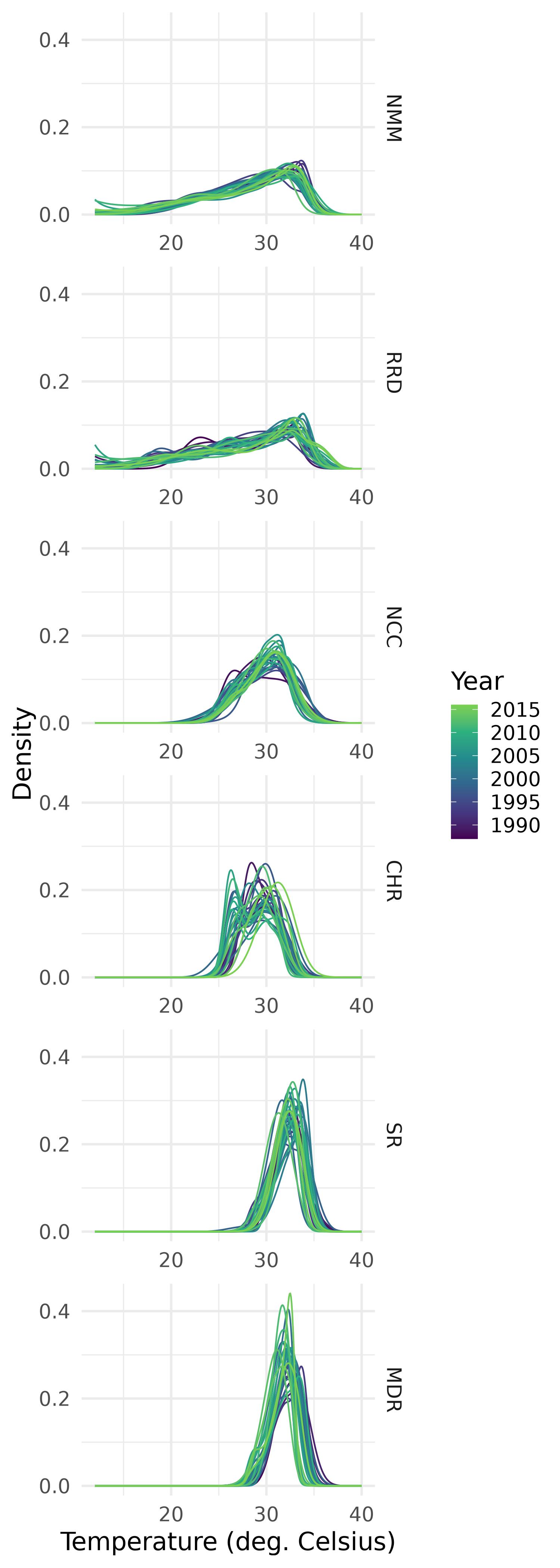
As in J. Machalová, Hron, and Monti (2016), after summarizing the initial temperature samples using histograms, penalized least squares splines are applied to smooth the data, treating the histogram bin centers as the first coordinates and the corresponding relative frequencies as the second coordinates. Figure 2, which displays the province-level temperature densities grouped by region, highlights distinct regional patterns in the temperature distributions.

Figure 2: Densities of maximum temperature across the years 1987 to 2016.

4.3 Temporal trends by province

To capture the temporal evolution of temperature density distributions across provinces within a given region (or within the whole Vietnam), we consider a simplified trend model in which each province’s density evolves linearly over time in the Bayes space sense. More precisely, if \(\pi_{gj}^{t}\) now denotes the density in province \(i\) (\(i=1,\ldots, n\)) at time \(t\), the simple time evolution model (for each province) is the following density-on-scalar regression model: \[\pi_{gj}^{t}(x)= [\alpha_{gj} \oplus ((t -t_0)\odot \beta_{gj}) \oplus \varepsilon_{gj}^{t}] (x), \tag{27}\] where \(t_0 = 1987\) is the first observed date, \(\beta_{gj}\) is the trend slope density (or simply slope density) for province \(i\) in region \(g\). The intercept \(\alpha_{gj}\) is the theoretical density for province \(j\) at time \(t=t_0.\) When the slope density of this model is the uniform distribution on \((a,b)\), there is no observable trend in the evolution of temperature densities.

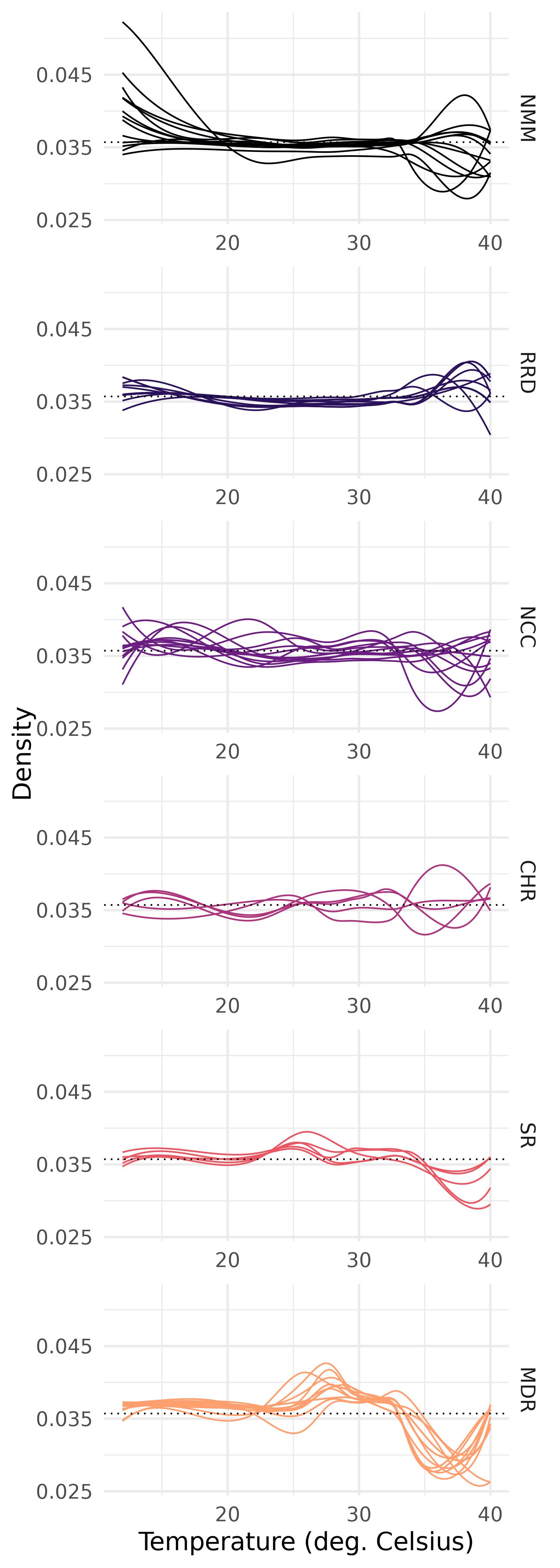
For estimating the parameters of Equation 27, as in R. Talská et al. (2018), the clr transformation is applied to Equation 27 and the resulting equation is that of a simple multivariate regression model which can be fitted by ordinary least squares. The fitted slopes seem to give a good approximation of the trend evolution since the coefficients of determination (defined in the context of density-on-scalar regression in R. Talská et al. 2018, 79) range from \(63\%\) to \(97\%\) (median of \(94\%\)) across provinces, with a better fit in the south. As often done in functional data, we will treat the resulting estimators of \(\alpha_{gj}\) and \(\beta_{gj}\) as our sample density dataset (and therefore do not use the hat notation). In Section 3.4, we also use the trend density functions \({\tilde \pi}_{gj}\) of this model defined by \[{\tilde \pi}_{gj}^{t}(x) = [{\alpha}_{gj} \oplus (t\odot {\beta}_{gj})](x). \tag{28}\] Figure 3 displays the province specific slope densities \({\beta}_{gj}\) grouped by region.

Figure 3: Trends slopes of provinces grouped by region. The dotted line represents the uniform density on \([12^\circ\text C, 40^\circ\text C]\) which is the reference measure.

In order to use our methodology, we will assume from now on that the \(\beta_{gj}\) are independent. Using the tools introduced by Menafoglio, Guadagnini, and Secchi (2014), we evaluated the spatial dependence between the slope densities and found it negligible.

4.4 Regional one-sample tests

Before testing the equality of trends between regions, it may be interesting to perform a one-sample test in each region separately to see whether there are some regions which are not affected by climate change. For a given region \(g\), we perform the one-sample test for the trend slope sample of \(\beta_{gj}\) for provinces \(j\) in region \(g\). To evaluate the existence of climate change, we choose \(\varphi_0\) to be the neutral element (uniform density in the interval \([12,40]\)), so that in each region, the null hypothesis represents the absence of temperature density change. The corresponding Šidák-adjusted \(p\)-values (see Abdi 2010) are displayed in Table 1. This table strongly supports the existence of climate change in the Red River Delta (RRD) region and in the southern regions SR and MDR, the non-existence of climate change in the Central Highlands (CHR) region. The results are more contrasted in the Northern Midlands and Mountains (NMM) region and in the North Central Coast (NCC) region where the tests are either non-significant or very marginally significant. These results should be interpreted with caution due to the small sample size in each region.

Table 1: Šidák-adjusted \(p\)-values for the regional one sample test.

region	PC	Norm
NMM	7.9e-02 *	0.12
RRD	1.6e-10 ***	1.5e-04 ***
NCC	8e-02 *	0.12
CHR	0.65	0.99
SR	1.8e-03 ***	4.2e-04 ***
MDR	0e+00 ***	4.9e-08 ***

4.5 Regional distributional ANOVA

Figure 4: Regional mean trend slopes. The dotted line represents the uniform density on \([12^\circ\text C, 40^\circ\text C]\) which is the reference measure.

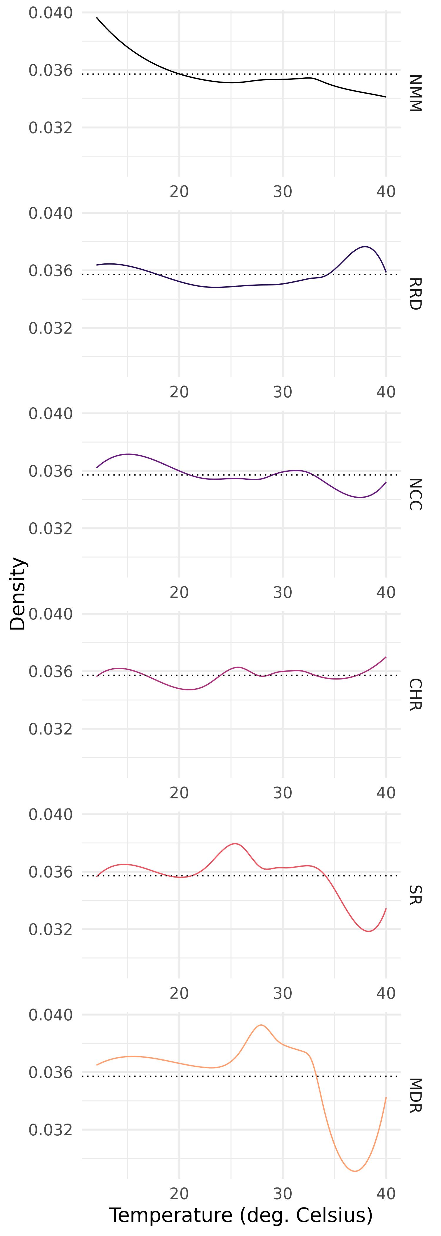
Figure 4 displays the regional mean trend slope densities. For the central regions (CHR and NCC), this plot shows a relative stability of the maximum temperature distribution (the trend is not far from uniform). For the RRD region, the curve exhibits a noticeable bump above the uniform on the right tail. More details about the interpretation of these curves will be given in Section 3.4.

Using the tests of Section 3.2 we now test whether these trend densities vary across regions. It is indeed important to evaluate the null hypotheses with different points of view due to the functional complex nature of the densities: group means can differ in many ways. Table 2 summarizes the results of the global analysis of variance for which the above tests all conclude that there is a difference in the way the regional temperature densities evolve in time.

Table 2: Test statistics and \(p\)-values for DANOVA.

Name	Statistic	p-value
GPF	10	0e+00 ***
Fmaxb	36	0e+00 ***
CS	700	0e+00 ***
L2B	130	0e+00 ***
FB	9.9	0e+00 ***

4.6 Pairwise comparisons between regions

Table 3 displays the tests statistics with their Šidák-adjusted \(p\)-values for the five pairwise tests. We summarize and visualize these results on Figure 5 by drawing

1. a solid line between two regions when none of the five tests reject the equality of mean slope densities
2. a dotted line between two regions when the equality of mean slope densities is rejected by some but not all of the five tests
3. no line between two regions when the equality of mean slope densities is rejected by all five tests.

At the exception of four dotted lines among the fifteen possible pairs, the large number of solid lines and “no line” supports the fact that the five tests agree most of the time. Note that the statistics GPF and \(F_{\max}\) agree in all cases but one. Among the statistics \(\operatorname{L^2B}\), FB and CS, there is at most one disagreement between pairs.

The structure of Figure 5 is interestingly similar to the geographical structure of the regions (see the map on Figure 1) with solid lines between neighboring regions. It shows that the Mekong Delta region differs statistically from most other regions in terms of climate change. Among the remaining regions, the Red River Delta region differs the most from the others in the sense that it is only connected by dotted lines.

Table 3: Šidák-adjusted \(p\)-values for pairwise group mean comparison.

region1	region2	GPF	Fmaxb	CS	L2B	FB
NMM	RRD	0.33	0.85	0e+00 ***	1e-01 *	0.18
NMM	NCC	1	0.97	1	1	1
NMM	CHR	0.48	0.37	0.96	0.97	0.99
NMM	SR	3e-05 ***	0e+00 ***	0.26	0.71	0.83
NMM	MDR	0e+00 ***	0e+00 ***	0e+00 ***	5.4e-09 ***	1.4e-06 ***
RRD	NCC	2.8e-02 **	0e+00 ***	0e+00 ***	2.5e-03 ***	8.6e-03 ***
RRD	CHR	3.3e-02 **	0e+00 ***	1	0.82	0.89
RRD	SR	0e+00 ***	0e+00 ***	0e+00 ***	8.7e-11 ***	3.9e-06 ***
RRD	MDR	0e+00 ***	0e+00 ***	0e+00 ***	0e+00 ***	0e+00 ***
NCC	CHR	0.98	0.96	0.99	0.99	1
NCC	SR	0.49	0.14	0.14	0.6	0.71
NCC	MDR	2e-13 ***	0e+00 ***	0e+00 ***	7.9e-13 ***	2.6e-09 ***
CHR	SR	0.27	0.54	0.46	0.15	0.4
CHR	MDR	4.8e-11 ***	0e+00 ***	0e+00 ***	3.7e-11 ***	2.3e-07 ***
SR	MDR	2.7e-06 ***	0.14	0e+00 ***	9e-04 ***	6.2e-03 ***

flowchart TB
  NMM([NMM]) ~~~ MDR([MDR])
  NMM <-.-> SR([SR])
  NMM <--> CHR([CHR]) <--> SR
  NMM <-.-> RRD([RRD]) <-.-> CHR
  RRD <--> NCC
  NCC <--> CHR
  NMM <--> NCC([NCC]) <--> SR
  SR <-.-> MDR
  NMM ~~~ MDR([MDR])

style NMM fill:#000004,color:#fff,stroke:#000
style RRD fill:#29115b,color:#fff,stroke:#000
style NCC fill:#6d1c82,color:#fff,stroke:#000
style CHR fill:#ac337b,stroke:#000
style SR fill:#ea5662,stroke:#000
style MDR fill:#ff9f6f,stroke:#000

Figure 5: Summary of pairwise tests between regions of Vietnam. Solid line: no test rejects the null hypothesis; dotted line: some tests reject the null hypothesis; absence of line: all tests reject the null hypothesis.

4.7 Interpreting regional changes in temperature distributions

Averaging Equation 28 over the province index for a given region \(g\), we get the regional trend density \[{\tilde \pi}_{g.}^{t}(x) = [{\alpha}_{g.} \oplus (t\odot {\bar \beta}_{g.})](x), \tag{29}\] and therefore the negative perturbation between two consecutive (between time \(t\) and \(t+1\)) trend density functions is constant equal to the regional slope density \(\bar\beta_{g.}.\) Hence as in Section 3.4, we can relate the relative frequency of \(\beta_{g.}\) at two temperature points \(x\) and \(z\) to the infinitesimal odds ratio of \({\tilde \pi}_{g.}^{t+1}\) versus \({\tilde \pi}_{g.}^{t}\)

Figure 6: Mean slope densities of North Central Coast (NCC) and Northern Midlands and Mountains (NMM) regions with levels.

Table 4: Levels for North Central Coast (NCC) and Northern Midlands and Mountains (NMM) regions.

region	x	y
NMM	21.5	0.0354
NMM	22.6	0.0353
NMM	27.6	0.0353
NMM	33.5	0.0353
NMM	34.1	0.0351
NCC	19.9	0.0360
NCC	21.0	0.0357
NCC	29.1	0.0357
NCC	32.9	0.0357
NCC	33.7	0.0354

Figure 7: Mean slope densities of Red River Delta (RRD) and Central Highlands (CHR) regions with levels.

Table 5: Levels for Red River Delta (RRD) and Central Highlands (CHR) regions.

region	x	y
RRD	35.6	0.0365
RRD	39.7	0.0365
RRD	17.3	0.0359
RRD	34.6	0.0359
CHR	38.7	0.0363
CHR	17.5	0.0355
CHR	23.5	0.0355

Figure 8: Mean slope densities of Southeast (SR) and Mekong Delta (MDR) regions with levels.

Table 6: Levels for Southeast (SR) and Mekong Delta (MDR) regions.

region	x	y
SR	22.9	0.0365
SR	27.5	0.0365
SR	34.2	0.0356
MDR	25.5	0.0371
MDR	32.6	0.0371
MDR	33.0	0.0363

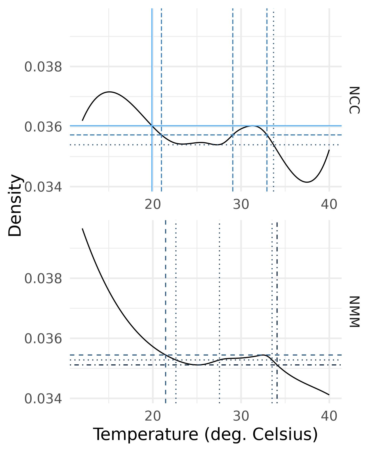
Figure 6, Figure 7 and Figure 8 display the slope densities of the six regions with some chosen values of level \(\tau\). We are able to group the regions in terms of the shape of their mean slope density.

On Figure 6 for northern regions, we select some levels \(\tau\) of the regional slope density \(\beta_{g.}\) and picture them on the graph: they are chosen so as to divide the full range (alternatively part of it) into two subintervals where the slope density is above (respectively below) that level or the reverse. For the NCC region for example, the highest level separates the temperature range into temperatures below 20\(^\circ\text C\) and temperatures above 20\(^\circ\text C\). The corresponding curve \(\beta_{g.}\) is above the chosen level for low temperatures and below for temperatures higher than 20\(^\circ\text C\), therefore by Equation 22 we may conclude that there is an increase of the frequency of low temperatures over time. Note that all levels higher than the previous one lead to the same conclusion. Similarly, the lowest level of \(\tau\) reveals a decrease of values of temperature approximately above \(33.7^\circ\text C\). Focusing now solely on the medium range between 21\(^\circ\text C\) and 33\(^\circ\text C\), the intermediate level separates the medium range into the interval \([21^\circ\text C,29.1^\circ\text C]\) where the slope density is below the level and its complement (within the medium range) where the slope density is above the level. We can conclude that in the medium range there is a shift towards higher temperatures over time. The same conclusion holds for the NMM region for which the medium range is \([22.6^\circ\text C,27.6^\circ\text C]\).

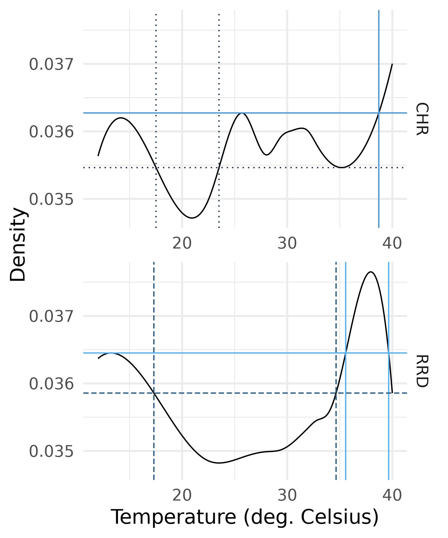
With the same strategy, based on Figure 7, we can see that the RRD region displays an increasing spread of its temperature distribution over time (values of \(\tau\) below the lowest level) and an increase of extremely high temperature events (values of \(\tau\) above the highest level). Note that since temperature change is not detected in the CHR region (Table 2), its interpretation based on odds ratio is probably not reliable.

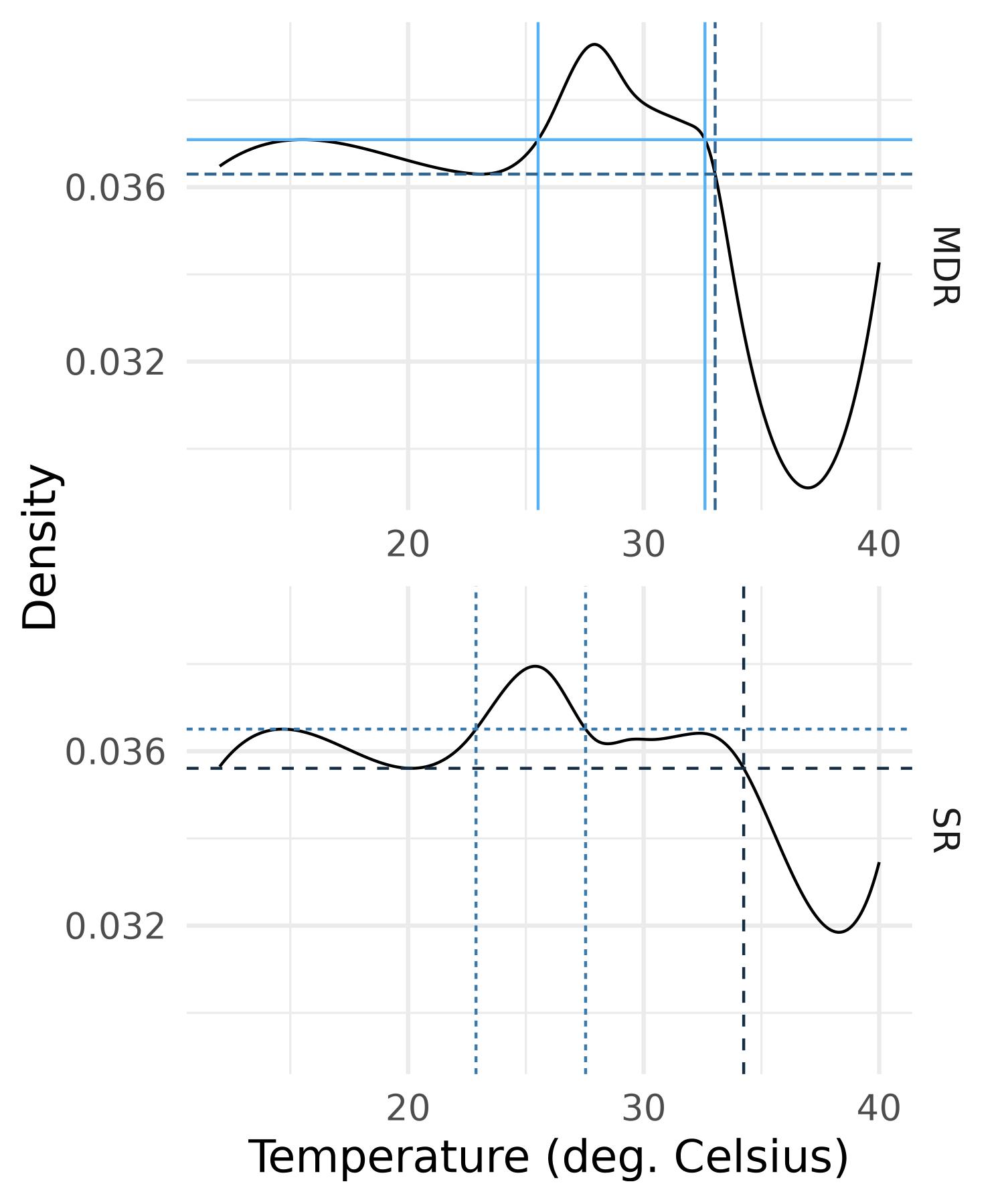
Based on Figure 8, the south in contrast shows a concentration in the medium range around 25\(^\circ\text C\) for SR and 28\(^\circ\text C\) for MDR at the expense of high temperatures.

While these groups reflect the geography (latitude and elevation) of Vietnam, they are also consistent with the groups suggested by the regional one-sample tests (Table 1) and the pairwise comparisons (Table 3).

5 Conclusion

We have adapted several functional data analysis tests to density functions in order to assess the equality of mean densities and to perform DANOVA tests in the framework of Bayes spaces. In our target application of temperature density evolution in Vietnam, the one-sample test allows to conclude that there is statistical evidence of the existence of climate change in Vietnam in the sense that the trend slope density is not uniform. Furthermore, when considering the functions globally, most of the DANOVA statistics strongly reject the null hypothesis, that is, the equality of trend slope density across the Vietnamese regions. For more local interpretations, we rely on the infinitesimal odds ratio of Maier et al. (2025).

Needless to say that the proposed methodology can be applied in other application frameworks. In our application, the inference has been carried out without taking into account the fact that the slope distributions are estimated with a linear model from data rather than observed. An alternative solution for testing the uniformity of climate change across regions would be to use a linear model for explaining the densities by time and a regional effect and to test the parameters of this model. In order to take into account the possible spatial dependence of the data set studied in this article, we could consider adapting the Spatial FANOVA methodology introduced by Aristizabal, Giraldo, and Mateu (2019) to a distributional context.

Future research might try to reduce the uncertainty due to the low density of extreme temperatures, possibly weighting the domain of the Bayes space as in Renáta Talská et al. (2020). Our local investigations remain exploratory, and elevating them to formal tests presents an interesting avenue for future research.

Our methodology is promising for environmental studies, with a possible application for example to the relative concentrations of contaminants in grounds or rivers analyzed as density functions.

Acknowledgments

Part of this work was completed while the authors were visiting the Vietnam Institute for Advanced Study in Mathematics (VIASM) in Hanoi and the authors express their gratitude to VIASM. We also acknowledge funding from the French National Research Agency (ANR) under grant ANR-17-EURE-0010 (Investissements d’Avenir program), from the French National Association of Research and Technology (ANRT), grant CIFRE n°2020/0011, and from Spanish Ministerio de Ciencia e Innovación grant number PID2021-123833OB-I00.

References

Abdi, Hervé. 2010. “Holm’s Sequential Bonferroni Procedure.” In Encyclopedia of Research Design, 574–77. SAGE Publications, Inc. https://doi.org/10.4135/9781412961288.

Aneiros, Germán, Ivana Horová, Marie Hušková, and Philippe Vieu. 2022. “On Functional Data Analysis and Related Topics.” Journal of Multivariate Analysis 189 (May): 104861. https://doi.org/10.1016/j.jmva.2021.104861.

Aristizabal, Jeimy-Paola, Ramón Giraldo, and Jorge Mateu. 2019. “Analysis of Variance for Spatially Correlated Functional Data: Application to Brain Data.” Spatial Statistics 32 (August): 100381. https://doi.org/10.1016/j.spasta.2019.100381.

Cuevas, Antonio, Manuel Febrero, and Ricardo Fraiman. 2004. “An Anova Test for Functional Data.” Computational Statistics & Data Analysis 47 (1): 111–22. https://doi.org/10.1016/j.csda.2003.10.021.

Egozcue, J. J., J. L. Díaz–Barrero, and V. Pawlowsky–Glahn. 2006. “Hilbert Space of Probability Density Functions Based on Aitchison Geometry.” Acta Mathematica Sinica, English Series 22 (4): 1175–82. https://doi.org/10.1007/s10114-005-0678-2.

Espagne, Etienne, Yoro Diallo, and Sébastien Marchand. 2019. “Impacts of Extreme Climate Events on Technical Efficiency in Vietnamese Agriculture.” Agence française de développement. https://ideas.repec.org//p/avg/wpaper/en9476.html.

Górecki, Tomasz, and Lukasz Smaga. 2018. “fdANOVA: Analysis of Variance for Univariate and Multivariate Functional Data.” https://cran.r-project.org/web/packages/fdANOVA/index.html.

———. 2019. “fdANOVA: An R Software Package for Analysis of Variance for Univariate and Multivariate Functional Data.” Computational Statistics 34 (2): 571–97. https://doi.org/10.1007/s00180-018-0842-7.

Gubler, Stefanie, Sophie Fukutome, and Simon C. Scherrer. 2023. “On the Statistical Distribution of Temperature and the Classification of Extreme Events Considering Season and Climate Change—an Application in Switzerland.” Theoretical and Applied Climatology 153 (3-4): 1273–91. https://doi.org/10.1007/s00704-023-04530-0.

Hron, K., A. Menafoglio, M. Templ, K. Hrůzová, and P. Filzmoser. 2016. “Simplicial Principal Component Analysis for Density Functions in Bayes Spaces.” Computational Statistics & Data Analysis 94 (February): 330–50. https://doi.org/10.1016/j.csda.2015.07.007.

Hsiang, Solomon, Robert Kopp, Amir Jina, James Rising, Michael Delgado, Shashank Mohan, D. J. Rasmussen, et al. 2017. “Estimating Economic Damage from Climate Change in the United States.” Science 356 (6345): 1362–69. https://doi.org/10.1126/science.aal4369.

Hultgren, Andrew, Tamma Carleton, Michael Delgado, Diana R. Gergel, Michael Greenstone, Trevor Houser, Solomon Hsiang, et al. 2022. “Estimating Global Impacts to Agriculture from Climate Change Accounting for Adaptation.” SSRN Electronic Journal. https://doi.org/10.2139/ssrn.4222020.

Kokoszka, Piotr, and Matthew Reimherr. 2017. Introduction to Functional Data Analysis. 1st ed. Chapman; Hall/CRC. https://doi.org/10.1201/9781315117416.

Machalová, J., K. Hron, and G. S. Monti. 2016. “Preprocessing of Centred Logratio Transformed Density Functions Using Smoothing Splines.” Journal of Applied Statistics 43 (8): 1419–35. https://doi.org/10.1080/02664763.2015.1103706.

Machalová, Jitka, Renáta Talská, Karel Hron, and Aleš Gába. 2021. “Compositional Splines for Representation of Density Functions.” Computational Statistics 36 (2): 1031–64. https://doi.org/10.1007/s00180-020-01042-7.

Maier, Eva-Maria, Almond Stöcker, Bernd Fitzenberger, and Sonja Greven. 2024. “Additive Density-on-Scalar Regression in Bayes Hilbert Spaces with an Application to Gender Economics.” arXiv. https://doi.org/10.48550/arXiv.2110.11771.

———. 2025. “Additive Density-on-Scalar Regression in Bayes Hilbert Spaces with an Application to Gender Economics.” The Annals of Applied Statistics 19 (1): 680–700. https://doi.org/10.1214/24-AOAS1979.

Martín-Fernández, Josep-Antoni, Josep Daunis-i-Estadella, and Glòria Mateu-Figueras. 2015. “On the Interpretation of Differences Between Groups for Compositional Data.” SORT-Statistics and Operations Research Transactions 39 (2): 231–52. https://raco.cat/index.php/SORT/article/view/302261.

Menafoglio, Alessandra, Alberto Guadagnini, and Piercesare Secchi. 2014. “A Kriging Approach Based on Aitchison Geometry for the Characterization of Particle-Size Curves in Heterogeneous Aquifers.” Stochastic Environmental Research and Risk Assessment 28 (7): 1835–51. https://doi.org/10.1007/s00477-014-0849-8.

Petersen, Alexander, Chao Zhang, and Piotr Kokoszka. 2022. “Modeling Probability Density Functions as Data Objects.” Econometrics and Statistics 21 (January): 159–78. https://doi.org/10.1016/j.ecosta.2021.04.004.

Ramsay, J. O., and B. W. Silverman. 2005. Functional Data Analysis. Springer Series in Statistics. New York, NY: Springer. https://doi.org/10.1007/b98888.

Roberts, Michael J., Wolfram Schlenker, and Jonathan Eyer. 2013. “Agronomic Weather Measures in Econometric Models of Crop Yield with Implications for Climate Change.” American Journal of Agricultural Economics 95 (2): 236–43. https://doi.org/10.1093/ajae/aas047.

Schlenker, Wolfram, and Michael J. Roberts. 2009. “Nonlinear Temperature Effects Indicate Severe Damages to U.S. Crop Yields Under Climate Change.” Proceedings of the National Academy of Sciences 106 (37): 15594–98. https://doi.org/10.1073/pnas.0906865106.

Schumaker, Larry. 1981. Spline Functions: Basic Theory. 3rd ed. Cambridge University Press. https://doi.org/10.1017/CBO9780511618994.

Shen, Qing, and Julian Faraway. 2004. “An F Test for Linear Models with Functional Responses.” Statistica Sinica 14 (4): 1239–57. https://www.jstor.org/stable/24307230.

Talská, Renáta, Alessandra Menafoglio, Karel Hron, Juan José Egozcue, and Javier Palarea‐Albaladejo. 2020. “Weighting the Domain of Probability Densities in Functional Data Analysis.” Stat 9 (1): e283. https://doi.org/10.1002/sta4.283.

Talská, R., A. Menafoglio, J. Machalová, K. Hron, and E. Fišerová. 2018. “Compositional Regression with Functional Response.” Computational Statistics & Data Analysis 123 (July): 66–85. https://doi.org/10.1016/j.csda.2018.01.018.

Tran, Trong Dinh, and Thang Van Nguyen. 2021. Climate Change Adaptation in Vietnam." In Climate Change Adaptation in Southeast Asia. Singapore: Springer Singapore.

Trinh, Huong Thi, Christine Thomas-Agnan, and Michel Simioni. 2023. “Scalar-on-Distribution Regression for Assessing the Impact of Climate Change on Rice Yield in Vietnam.” TSE Working Paper 23-1410 (February). https://www.tse-fr.eu/sites/default/files/TSE/documents/doc/wp/2023/wp_tse_1410.pdf.

Trinh, Trong Anh. 2018. “The Impact of Climate Change on Agriculture: Findings from Households in Vietnam.” Environmental and Resource Economics 71 (4): 897–921. https://doi.org/10.1007/s10640-017-0189-5.

Trinh, Trong-Anh, Simon Feeny, and Alberto Posso. 2021. “The Impact of Natural Disasters and Climate Change on Agriculture: Findings From Vietnam.” In Economic Effects of Natural Disasters, 261–80. Elsevier. https://doi.org/10.1016/B978-0-12-817465-4.00017-0.

Van Den Boogaart, Karl Gerald, J. J. Egozcue, and Vera Pawlowsky-Glahn. 2010. “Bayes Linear Spaces.” SORT : Statistics and Operations Research Transactions 34 (December): 201–22.

Van Den Boogaart, Karl Gerald, Juan José Egozcue, and Vera Pawlowsky-Glahn. 2014. “Bayes Hilbert Spaces.” Australian & New Zealand Journal of Statistics 56 (2): 171–94. https://doi.org/10.1111/anzs.12074.

Vo, Trung Hung, Viet Thanh Nguyen, and Michel Simioni. 2022. “Adaptation of Rice Yields to Heat Stress in Vietnam: New Insight from Heterogeneous Slopes Panel Data Modeling.” In. https://hal.inrae.fr/hal-03715498.

World Bank Group, and Asian Development Bank. 2021. Climate Risk Country Profile: Vietnam. World Bank. https://doi.org/10.1596/36367.

World Meteorological Organization. 2023. “The Global Climate 2011-2020: A Decade of Acceleration.” World Meteorological Organization. https://wmo.int/publication-series/global-climate-2011-2020-decade-of-acceleration.

———. 2024. “State of the Global Climate 2023.” WMO-No. 1347. World Meteorological Organization. https://wmo.int/publication-series/state-of-global-climate-2023.

Zhang, Jin-Ting. 2011. “Statistical Inferences for Linear Models with Functional Responses.” Statistica Sinica 21 (3): 1431–51. https://doi.org/10.5705/ss.2009.302.

———. 2013. Analysis of Variance for Functional Data. 0th ed. Chapman; Hall/CRC. https://doi.org/10.1201/b15005.

Zhang, Jin-Ting, and Jianwei Chen. 2007. “Statistical Inferences for Functional Data.” The Annals of Statistics 35 (3): 1052–79. https://doi.org/10.1214/009053606000001505.

Zhang, Jin-Ting, Ming-Yen Cheng, Hau-Tieng Wu, and Bu Zhou. 2019. “A New Test for Functional One-Way ANOVA with Applications to Ischemic Heart Screening.” Computational Statistics & Data Analysis 132 (April): 3–17. https://doi.org/10.1016/j.csda.2018.05.004.

Zhang, Jin-Ting, and Xuehua Liang. 2014. “One-Way ANOVA for Functional Data via Globalizing the Pointwise F-Test.” Scandinavian Journal of Statistics 41 (1): 51–71. https://doi.org/10.1111/sjos.12025.