Outlier detection using ICS and climate change in Vietnam

library(dda)
library(tidyverse)
library(sf)
library(fdaoutlier)
library(DeBoinR)
library(tf)
if (!require(tidyfun)) {
  remotes::install_github("tidyfun/tidyfun")
  library(tidyfun)
}
set.seed(0)

4 years, 2 regions and 2 outliers (28 provinces)

In this toy example, we filter the dataset on Vietnam temperature to consider only the two northern regions and two provinces from the south, from 2013 to 2016, for a total of 112 observations. The aim is to study the influence of the preprocessing parameters.

Data presentation

data(vietnam_provinces)
data(vietnam_regions)

vietnam_provinces |>
  mutate(
    province = if_else(region %in% c("NMM", "RRD") | province %in% c("ANGIANG", "BACLIEU"), province, NA),
    region = if_else(region %in% c("NMM", "RRD", "MDR"), region, NA)
  ) |>
  left_join(vietnam_regions, by = c("region" = "code")) |>
  select(!region) |>
  rename(region = name) |>
  ggplot(aes(fill = region, label = province)) +
  geom_sf() +
  geom_sf_label(fill = "white", size = 3) +
  scale_fill_discrete(na.translate = FALSE) +
  scale_x_continuous(breaks = seq(from = -180, to = 180, by = 2)) +
  labs(x = "longitude", y = "latitude")

Map of Vietnam showing the 63 provinces, color-coded by region. The 28 provinces included in the toy example are labeled.

# Filter the data set
data(vietnam_temperature)
selected_years <- 2013:2016

vnt <- vietnam_temperature |>
  filter(year %in% selected_years) |>
  filter(region %in% c("NMM", "RRD") | province %in% c("ANGIANG", "BACLIEU")) |>
  left_join(vietnam_regions, by = c("region" = "code")) |>
  select(!region) |>
  rename(region = name) |>
  arrange(region, province)

vnts <- vnt |>
  mutate(t_max = as_dd(t_max,
    lambda = 1, nbasis = 12, mc.cores = 12
  ))

vnts |>
  plot_funs(t_max, color = region) +
  theme_legend_inside +
  labs(x = "temperature (deg. Celsius)", y = "density")

Densities of maximum temperature over 28 provinces of Vietnam and during the years 2013-2016, color-coded by region.

vnts |>
  mutate(t_max = as.fd(center(t_max))) |>
  plot_funs(t_max, color = region) +
  theme(legend.position = "none") +
  labs(x = "temperature (deg. Celsius)", y = "centred clr(density)")

Centred log-ratio transforms of the centred densities of maximum temperature over 28 provinces of Vietnam and during the years 2013-2016, color-coded by region.

vnts |>
  mutate(
    t_max = as.fd(t_max),
    year = ifelse(province == "LAICHAU", year, "not LAICHAU"),
    alpha = ifelse(province == "LAICHAU", 1, 0.85)
  ) |>
  plot_funs(t_max, color = year, alpha = alpha) +
  labs(x = "temperature (deg. Celsius)", y = "clr(density)") +
  guides(alpha = "none")

Centred log-ratio transforms of the densities of maximum temperature over 28 provinces of Vietnam and during the years 2013-2016. The case of LAICHAU.

Influence of the preprocessing parameters

Let us create a grid of parameters and define the function to call for each parameter.

smooth_ICS <- function(vnt, knots_pos, nknots, lambda, index) {
  vnts <- vnt |>
    mutate(t_max = as_dd(t_max,
      lambda = lambda, nbasis = 5 + nknots,
      mc.cores = parallel::detectCores() - 1, knots_pos = knots_pos
    ))
  knots_pos_str <- ifelse(knots_pos == "quantiles",
    "Knots at quantiles", "Equally spaced knots"
  )
  index_str <- ifelse(is.na(index), "Auto selection of components",
    paste("# of components:", index)
  )

  print(paste(
    "# of knots:", nknots, "|",
    "log10(lambda):", log10(lambda), "|",
    knots_pos_str, "|",
    index_str
  ))

  if (is.na(index)) {
    list(
      dd = vnts$t_max,
      ics = tryCatch(ICS(as.fd(vnts$t_max)), error = function(e) e),
      ics_out = tryCatch(ICS_outlier(as.fd(vnts$t_max),
        n_cores = parallel::detectCores() - 1
      ), error = function(e) e)
    )
  } else {
    list(
      dd = vnts$t_max,
      ics = tryCatch(ICS(as.fd(vnts$t_max)), error = function(e) e),
      ics_out = tryCatch(ICS_outlier(as.fd(vnts$t_max),
        n_cores = parallel::detectCores() - 1, index = seq_len(index)
      ), error = function(e) e)
    )
  }
}

knots_pos_seq <- c("quantiles", "equally spaced")
nknots_seq <- c(5:19, seq(20, 40, 10)) - 5
lambda_seq <- 10^(-8:8)
index_seq <- 4

param_grid <- expand.grid(
  knots_pos = knots_pos_seq,
  nknots = nknots_seq,
  lambda = lambda_seq,
  index = index_seq
) |>
  arrange(nknots, knots_pos, lambda)

knitr::kable(
  tibble(
    `# of knots positions` = length(knots_pos_seq),
    `# of # of knots` = length(nknots_seq),
    `# of values for lambda` = length(lambda_seq),
    `# of # of components` = length(lambda_seq),
    `# of values for index` = length(index_seq),
    `Total grid size` = nrow(param_grid)
  )
)

# of knots positions	# of # of knots	# of values for lambda	# of # of components	# of values for index	Total grid size
2	18	17	17	1	612

if (!file.exists("ICS_north_south_outliers.RData") && !file.exists("ICS_north_south.RData")) {
  system.time(
    ics_grid <- param_grid |>
      mutate(id = seq_len(n())) |>
      rowwise() |>
      mutate(res = list(smooth_ICS(vnt, knots_pos, nknots, lambda, index)))
  )
  save(ics_grid, file = "ICS_north_south.RData")
}

if (!file.exists("ICS_north_south_outliers.RData")) {
  load("ICS_north_south.RData")

  ics_grid_out <- ics_grid |>
    rowwise() |>
    filter(!(any(class(res$ics_out) == "error"))) |>
    mutate(res = list(data.frame(
      obs_id = seq_len(length((res$ics_out$outliers))),
      outlying = res$ics_out$outliers == 1,
      distance = res$ics_out$ics_distances
    ))) |>
    unnest(res)

  save(ics_grid_out, file = "ICS_north_south_outliers.RData")
}

load("ICS_north_south_outliers.RData")

ics_grid_out |>
  left_join(vnt |> mutate(obs_id = row_number()), by = c("obs_id")) |>
  filter(nknots %% 2 == 0 | nknots > 20) |>
  mutate(region = str_wrap(region, 25)) |>
  ggplot(aes(log10(lambda), obs_id, fill = region, alpha = outlying)) +
  geom_tile() +
  facet_grid(cols = vars(nknots), rows = vars(knots_pos)) +
  labs(y = "observation index")

Outlier detection using ICS on 28 provinces of Vietnam, during the years 2013-2016, over a grid of preprocessing parameters. Columns correspond to the number of inside knots (0-35).

ics_grid_summary <- ics_grid_out |>
  mutate(outlying = ifelse(outlying, 1, 0)) |>
  group_by(obs_id) |>
  summarise(n_outlying = sum(outlying), mean_distance = mean(distance)) |>
  left_join(vnt |> mutate(obs_id = row_number()), by = c("obs_id")) |>
  select(obs_id, region, province, year, n_outlying, mean_distance)

rmarkdown::paged_table(ics_grid_summary)

ics_grid_summary |>
  ggplot(aes(obs_id, n_outlying, fill = region)) +
  geom_bar(stat = "identity") +
  theme_legend_inside_right +
  labs(x = "observation index", y = "outlier detection frequency")

Summary of outlier detection using ICS on 28 provinces of Vietnam, during the years 2013-2016, over a grid of preprocessing parameters.

ics_grid_summary |>
  ggplot(aes(obs_id, mean_distance, fill = region)) +
  geom_bar(stat = "identity") +
  theme_legend_inside_right +
  labs(x = "observation index", y = "mean ICS distance")

Summary of outlier detection using ICS on 28 provinces of Vietnam, during the years 2013-2016, over a grid of preprocessing parameters.

30 years, 1 climate region (13 provinces)

Data presentation

vietnam_provinces <- vietnam_provinces |>
  arrange(region, province) |>
  mutate(climate_region = case_when(
    province %in% c("LAICHAU", "DIENBIEN", "SONLA") ~ "S1",
    province %in% c(
      "LAOCAI", "YENBAI", "HAGIANG", "CAOBANG", "TUYENQUANG",
      "BACKAN", "THAINGUYEN", "LANGSON", "BACGIANG", "QUANGNINH"
    ) ~ "S2",
    region %in% c("NMM", "RRD") ~ "S3",
    .default = NA
  ))

vietnam_provinces |>
  filter(region %in% c("RRD", "NMM")) |>
  ggplot(aes(fill = climate_region, label = province)) +
  geom_sf() +
  geom_sf_label(fill = "white") +
  scale_fill_viridis_d() +
  labs(x = "longitude", y = "latitude", fill = "climate region")

The three climate regions of northern Vietnam.

library(tidyverse)
library(sf)
data(vietnam_temperature)
data(vietnam_regions)
data(vietnam_provinces)

vntcr <- vietnam_temperature |>
  filter(region %in% c("RRD", "NMM")) |>
  dplyr::select(year, province, t_max) |>
  left_join(vietnam_provinces, by = "province") |>
  st_as_sf() |>
  dplyr::select(year, climate_region, province, t_max) |>
  filter(climate_region == "S3") |>
  arrange(year, province)

vnt <- vntcr |>
  mutate(t_max = as_dd(t_max, lambda = 10, nbasis = 10, mc.cores = 15))
class(vnt$t_max) <- c("ddl", "fdl", "list")

vnt |> plot_funs(t_max, color = province) +
  facet_wrap(vars(year)) +
  labs(x = "temperature (deg. Celsius)", y = "density")

Densities of maximum temperatures in the 13 provinces of the S3 climate region of Vietnam during the years 1987-2016.

Outlier detection using ICS

icsout <- ICS_outlier(vnt$t_max, index = 1:2, n_cores = 14)

icsout$result |> ggplot(aes(index, gen_kurtosis, group = 1)) +
  geom_line(alpha = 0.5) +
  geom_point(aes(color = index, alpha = selected), size = 3) +
  theme_legend_inside_right +
  labs(x = "", y = "ICS eigenvalues") +
  guides(color = "none")

Scree plot of ICS eigenvalues.

icsout$result |>
  filter(selected) |>
  plot_funs(H_dual, color = index) +
  geom_hline(yintercept = 1 / diff(icsout$result$H_dual[[1]]$basis$rangeval), linetype = "dotted") +
  labs(x = "temperature (deg. Celsius)", y = "density") +
  scale_color_manual(values = scales::pal_hue()(9)[1:2]) +
  theme_legend_inside

Dual ICS eigendensities.

h_dual_shift <- c(3 * icsout$result$H_dual)
h_dual_shift$coefs <- sweep(h_dual_shift$coefs, 1, -c(mean(vnt$t_max))$coefs)
icsout$result |>
  mutate(H_dual_shift = as.list(h_dual_shift)) |>
  filter(selected) |>
  plot_funs(H_dual_shift, color = index) +
  geom_function(fun = function(x) eval(c(mean(vnt$t_max)), x), color = "black", linetype = "dotted") +
  scale_color_manual(values = scales::pal_hue()(9)[1:2]) +
  labs(x = "temperature (deg. Celsius)", y = "density") +
  theme_legend_inside

Shifting the mean in the direction of each dual ICS eigendensity.

vnt <- vnt |>
  mutate(
    index = seq_len(nrow(icsout$scores)),
    outlying = as.factor(icsout$outliers),
    distances = icsout$ics_distances
  ) |>
  cbind(icsout$scores)

vnt |>
  mutate(year = as.factor(ifelse(outlying == 1, year, NA))) |>
  arrange(outlying) |>
  plot_funs(t_max, color = year, alpha = outlying) +
  theme_legend_inside +
  labs(
    x = "temperature (deg. Celsius)", y = "density",
    color = "outlying\nyears"
  ) +
  scale_color_discrete(limits = function(x) ifelse(is.na(x), "", x)) +
  guides(alpha = "none")

Outlying densities of maximum temperature in the provinces of the S3 climate region of Vietnam during the years 1987-2016.

vnt |>
  mutate(
    t_max = as.fd(center(t_max)),
    year = as.factor(ifelse(outlying == 1, year, NA))
  ) |>
  arrange(outlying) |>
  plot_funs(t_max, color = year, alpha = outlying) +
  theme(legend.position = "none") +
  labs(
    x = "temperature (deg. Celsius)", y = "centred clr(density)",
    color = "outlying\nyears"
  )

Centred log-ratio transforms of the outlying centred densities of maximum temperature in the provinces of the S3 climate region of Vietnam during the years 1987-2016.

vnt |>
  mutate(province = ifelse(outlying == 1, province, NA)) |>
  arrange(outlying) |>
  plot_funs(t_max, color = province, alpha = outlying) +
  facet_wrap(vars(year)) +
  labs(
    x = "temperature (deg. Celsius)", y = "density",
    color = "outlying\nprovinces"
  ) +
  scale_color_discrete(limits = function(x) ifelse(is.na(x), "", x)) +
  guides(alpha = "none")

Outlying densities of maximum temperature in the provinces of the S3 climate region of Vietnam during the years 1987-2016.

vnt |>
  mutate(
    t_max = as.fd(center(t_max)),
    province = ifelse(outlying == 1, province, NA)
  ) |>
  arrange(outlying) |>
  plot_funs(t_max, color = province, alpha = outlying) +
  facet_wrap(vars(year)) +
  labs(
    x = "temperature (deg. Celsius)", y = "centred clr(density)",
    color = "outlying\nprovinces"
  ) +
  scale_color_discrete(limits = function(x) ifelse(is.na(x), "", x)) +
  guides(alpha = "none")

Centred log-ratio transforms of the outlying centred densities of maximum temperature in the provinces of the S3 climate region of Vietnam during the years 1987-2016.

vnt |>
  mutate(province = ifelse(outlying == 1, province, NA)) |>
  ggplot(aes(year, distances, color = province, label = year)) +
  geom_text() +
  scale_color_discrete(limits = function(x) ifelse(is.na(x), "", x)) +
  geom_hline(yintercept = icsout$ics_dist_cutoff) +
  labs(color = "outlying\nprovinces")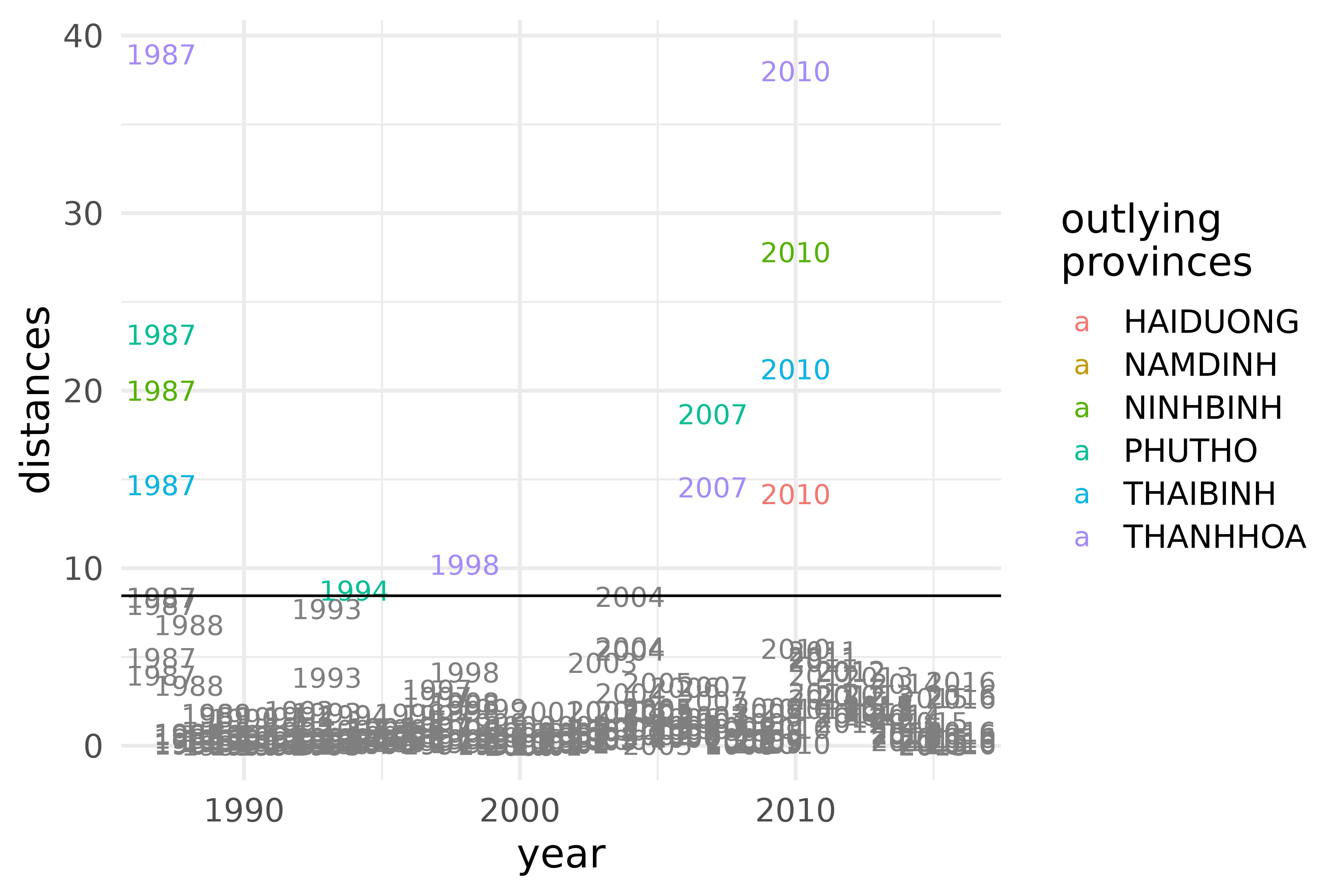

ICS distances of the densities of maximum temperature in the provinces of the S3 climate region of Vietnam during the years 1987-2016.

vnt |>
  mutate(province = ifelse(outlying == 1, province, NA)) |>
  ggplot(aes(IC.1, IC.2)) +
  scale_color_discrete(limits = function(x) ifelse(is.na(x), "", x)) +
  geom_text(aes(color = province, label = year)) +
  labs(color = "outlying\nprovinces")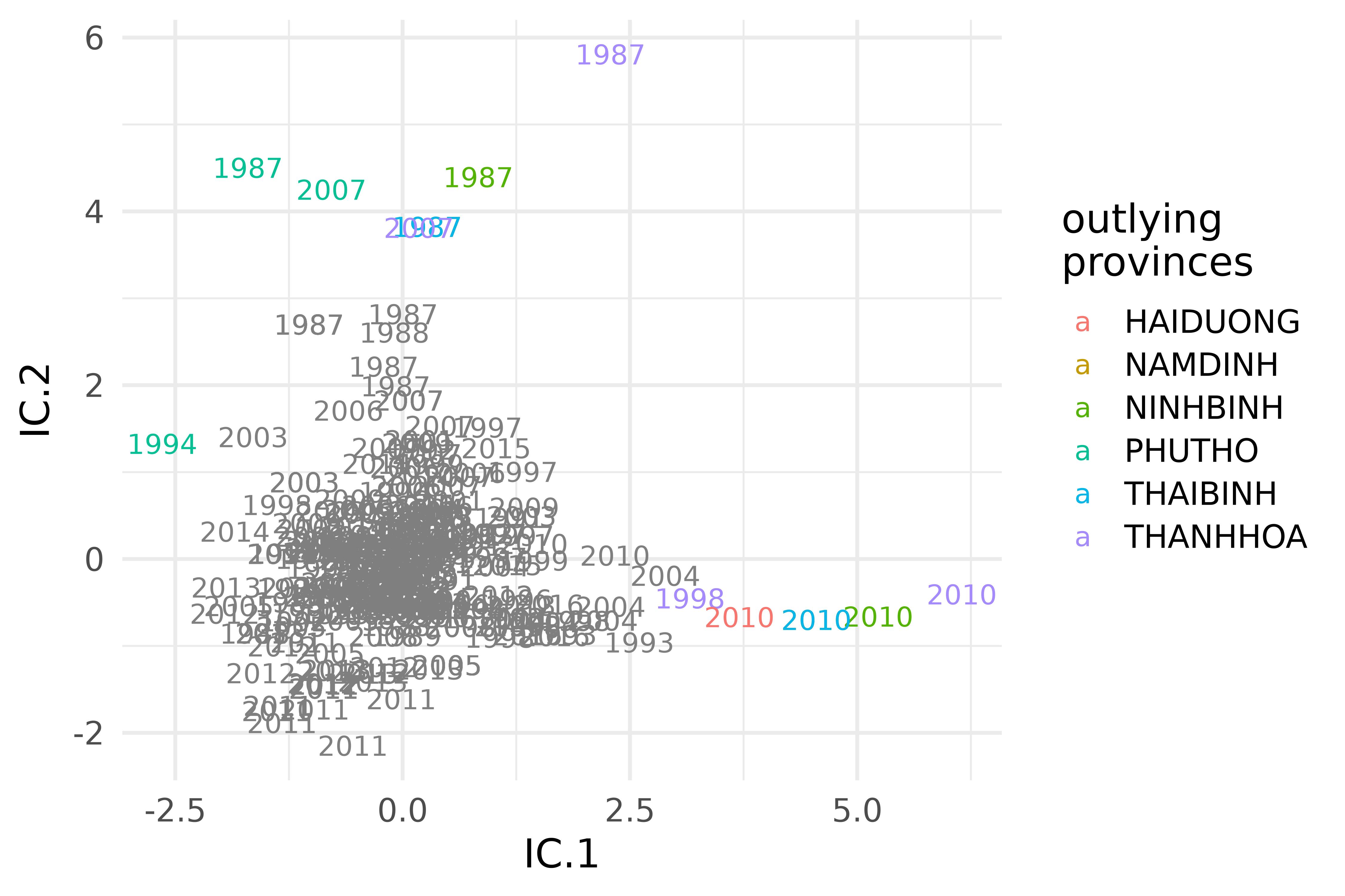

Selected invariant coordinates of the densities of maximum temperature in the provinces of the S3 climate region of Vietnam during the years 1987-2016.

Influence of the preprocessing parameters

Now let us apply ICS for outlier detection on the same dataset but with different smoothing parameters.

knots_pos_seq <- "quantiles"
nknots_seq <- 5 * 1:5
lambda_seq <- 10^(-2:2)
index_seq <- c(2, NA)

param_grid <- expand.grid(
  knots_pos = knots_pos_seq,
  nknots = nknots_seq,
  lambda = lambda_seq,
  index = index_seq
) |>
  arrange(nknots, knots_pos, lambda)

knitr::kable(
  tibble(
    `# of knots positions` = length(knots_pos_seq),
    `# of # of knots` = length(nknots_seq),
    `# of values for lambda` = length(lambda_seq),
    `# of # of components` = length(lambda_seq),
    `# of values for index` = length(index_seq),
    `Total grid size` = nrow(param_grid)
  )
)

# of knots positions	# of # of knots	# of values for lambda	# of # of components	# of values for index	Total grid size
1	5	5	5	2	50

if (!file.exists("ICS_climate_regions.RData")) {
  system.time(
    ics_grid <- param_grid |>
      mutate(id = seq_len(n())) |>
      rowwise() |>
      mutate(res = list(smooth_ICS(vntcr, knots_pos, nknots, lambda, index)))
  )
  save(ics_grid, file = "ICS_climate_regions.RData")
}

load("ICS_climate_regions.RData")

ics_grid_out <- ics_grid |>
  rowwise() |>
  filter(!(any(class(res$ics_out) == "error"))) |>
  mutate(res = list(data.frame(
    obs_id = seq_len(length((res$ics_out$outliers))),
    outlying = res$ics_out$outliers == 1
  ))) |>
  unnest(res)

ics_grid_out |>
  mutate(index = ifelse(is.na(index), "auto. selection of ICs",
    paste(index, "ICs selected")
  )) |>
  ggplot(aes(log10(lambda), obs_id, fill = outlying, alpha = outlying)) +
  geom_tile() +
  scale_fill_grey(start = 1, end = 0) +
  facet_grid(cols = vars(nknots), rows = vars(index)) +
  labs(y = "observation index")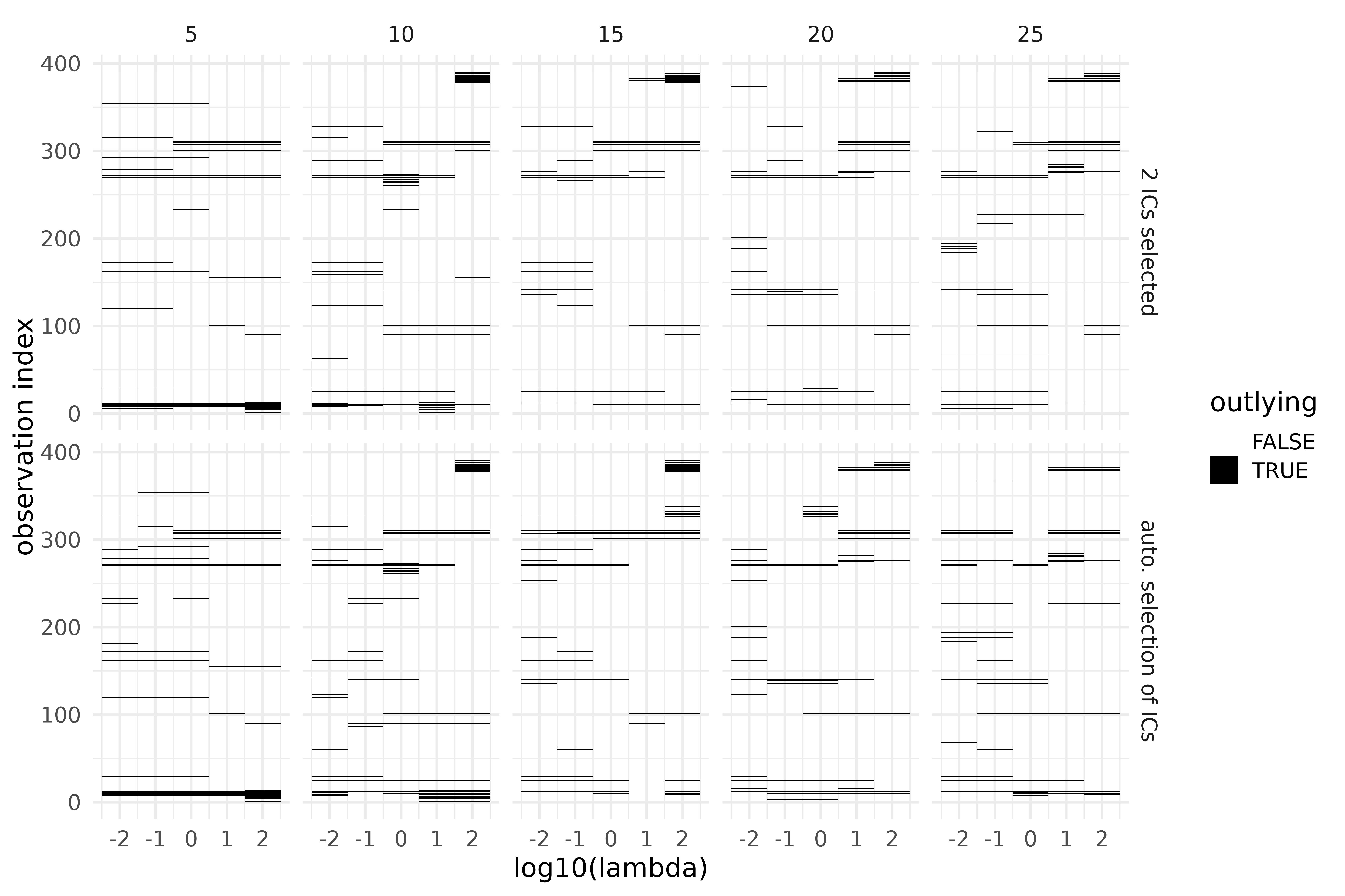

Outlier detection using ICS on the S3 climate region of Vietnam, during the years 1987-2016, over a grid of preprocessing parameters. Top: 2 invariant components selected; bottom: automatic selection through D’Agostino tests. Columns correspond to the number of inside knots (5-25).

ics_grid_out |>
  mutate(index = ifelse(is.na(index), "auto. selection of ICs",
    paste(index, "ICs selected")
  )) |>
  rename(index_select = index) |>
  left_join(vnt |> mutate(obs_id = row_number()) |> select(!outlying), by = c("obs_id")) |>
  group_by(nknots, lambda, index_select, year) |>
  mutate(n_outlying = sum(outlying) / 13) |>
  ggplot(aes(log10(lambda), year, fill = n_outlying, alpha = n_outlying)) +
  geom_tile() +
  scale_alpha_continuous(range = c(0, 1)) +
  scale_fill_gradient(low = "white", high = "black") +
  facet_grid(cols = vars(nknots), rows = vars(index_select)) +
  labs(y = "year", fill = "outlier\nfrequency", alpha = "") +
  guides(alpha = "none")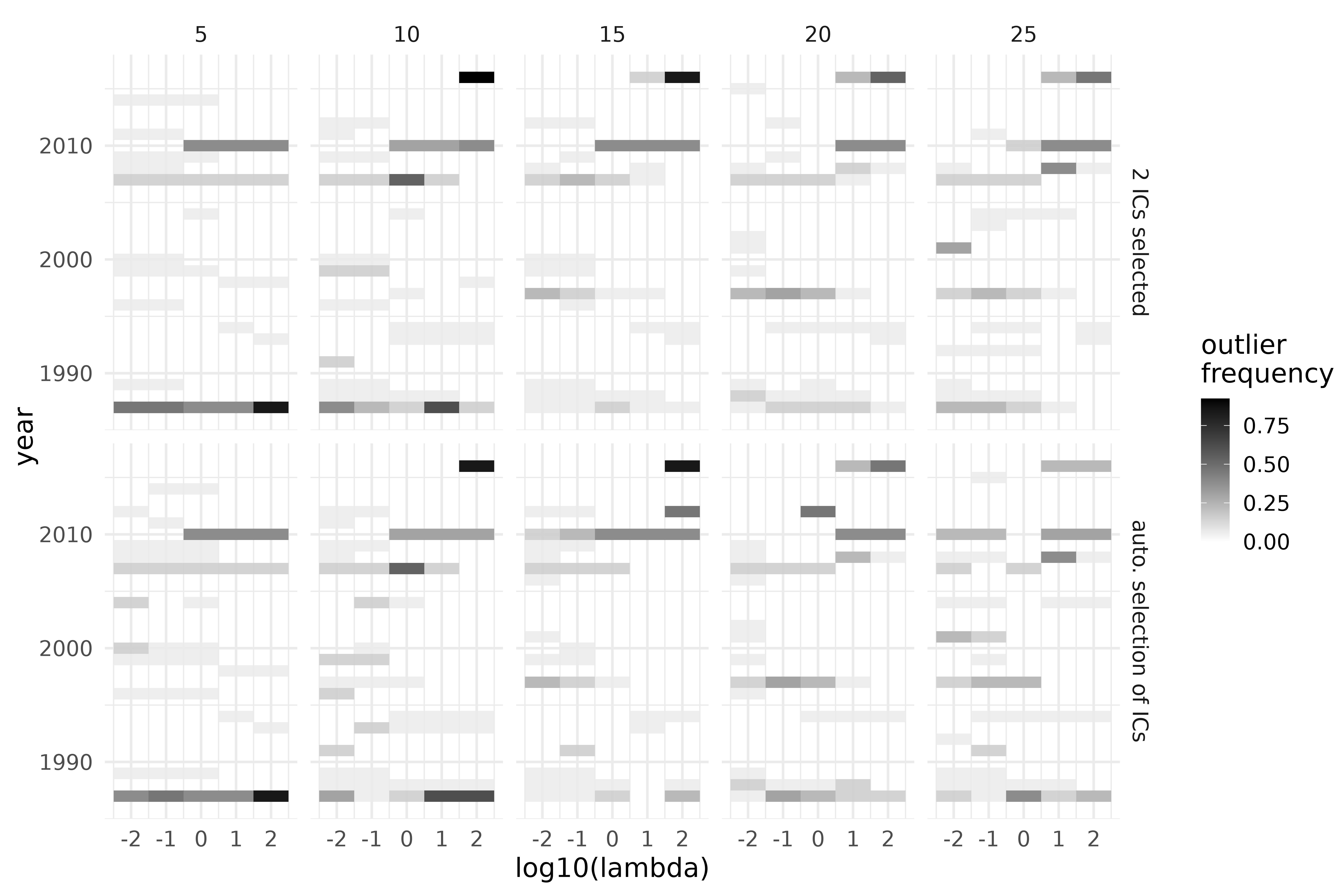

Outlier detection using ICS on the S3 climate region of Vietnam, during the years 1987-2016, over a grid of preprocessing parameters. Top: 2 invariant components selected; bottom: automatic selection through D’Agostino tests. Columns correspond to the number of inside knots (5-25).

ics_grid |>
  filter(is.na(index)) |>
  mutate(`number of selected ICs` = max(res$ics_out$index)) |>
  ggplot(aes(log10(lambda), `number of selected ICs`)) +
  geom_bar(stat = "identity") +
  facet_grid(cols = vars(nknots))

Outlier detection using ICS on the S3 climate region of Vietnam, during the years 1987-2016, over a grid of preprocessing parameters. Top: 2 invariant components selected; bottom: automatic selection through D’Agostino tests. Columns correspond to the number of inside knots (5-25).

ics_grid_summary <- ics_grid_out |>
  mutate(outlying = ifelse(outlying, 1, 0)) |>
  group_by(obs_id) |>
  summarise(n_outlying = sum(outlying)) |>
  left_join(vnt |> mutate(obs_id = row_number()), by = c("obs_id")) |>
  select(obs_id, province, year, n_outlying)

rmarkdown::paged_table(ics_grid_summary)

ics_grid_summary |>
  ggplot(aes(year, n_outlying)) +
  geom_bar(stat = "identity") +
  labs(y = "outlier detection frequency")

Outlier detection using ICS on the S3 climate region of Vietnam, during the years 1987-2016, over a grid of preprocessing parameters.

Constraining the centred log-ratio transforms to zero on the boundaries

If we force to 0 the first and last ZB-spline coordinates of the \(\operatorname{clr}\), we project them onto the space of splines constrained to \(0\) on the boundaries of the interval.

boundary_to_zero <- function(x) {
  b <- x$basis
  p <- b$nbasis
  zbsp <- fd(to_zbsplines(inv = TRUE, coefs = diag(p - 1), basis = b), b)
  plot(as.list(zbsp))

  y <- to_zbsplines(x)
  y[c(1, p - 1), ] <- 0
  yfd <- fd(to_zbsplines(inv = TRUE, coefs = y, basis = b), b)

  list(dd = yfd, coefs = t(y[2:(p - 2), ]))
}
icsout <- ICS_outlier(boundary_to_zero(c(vnt$t_max))$coefs)

vnt |>
  mutate(
    t_max = as.list(as.fd(boundary_to_zero(c(t_max))$dd)),
    outlying = icsout$outliers == 1,
    province = ifelse(outlying == 1, province, NA)
  ) |>
  plot_funs(t_max, color = province, alpha = outlying) +
  facet_wrap(vars(year)) +
  scale_color_discrete(limits = function(x) ifelse(is.na(x), "", x)) +
  labs(
    x = "temperature (deg. Celsius)", y = "clr(density)",
    color = "outlying\nprovinces"
  )

Outlier detection using ICS on the S3 climate region of Vietnam, with centred log-ratio transforms constrained to 0 on the boundaries.

Comparison with other methods

See this vignette from fdaoutlier for more details about simulation models.

schemes <- c("GP_clr", "Gumbel", "GP_margin")

simulation_gp_clr <- function(n, p) {
  sim <- fdaoutlier::simulation_model4(n, p, mu = 15, outlier_rate = 0.02)
  y <- exp(tfd(sim$data, arg = seq(0, 1, length.out = p)))

  list(
    data = as.matrix(y / tf_integrate(y)),
    true_outliers = replace(integer(n), sim$true_outliers, 1)
  )
}

dgumbel <- function(x, mu = 0, beta = 1) {
  z <- (x - mu) / beta
  exp(-z - exp(-z)) / beta
}

simulation_gumbel <- function(n, p, outlier_rate = 0.02, deterministic = TRUE) {
  tt <- seq(0, 1, length.out = p)
  a <- matrix(rnorm(n, sd = 0.01), nrow = p, ncol = n, byrow = TRUE)
  b <- matrix(rnorm(n, sd = 0.01), nrow = p, ncol = n, byrow = TRUE)
  y <- dgumbel(tt, mu = 0.25 + a, beta = 0.05 + b)
  dtt <- fdaoutlier:::determine(deterministic, n, outlier_rate)
  n_outliers <- dtt$n_outliers
  true_outliers <- dtt$true_outliers
  if (n_outliers > 0) {
    a <- matrix(rnorm(n_outliers, sd = 0.01),
      nrow = p, ncol = n_outliers, byrow = TRUE
    )
    b <- matrix(rnorm(n_outliers, sd = 0.01),
      nrow = p, ncol = n_outliers, byrow = TRUE
    )
    y[, true_outliers] <- dgumbel(tt, mu = 0.32 + a, beta = 0.05 + b)
  }
  rownames(y) <- tt
  return(list(
    data = t(y),
    true_outliers = replace(integer(n), true_outliers, 1)
  ))
}

simulation_gp_margin <- function(n, p) {
  sim <- fdaoutlier::simulation_model5(n, p, outlier_rate = 0.02)
  y <- tibble(f = split(sim$data, row(sim$data))) |>
    mutate(f = as_dd(f, lambda = 1, nbasis = 10, mc.cores = 14))
  tt <- seq(min(sim$data), max(sim$data), length.out = p)
  densities_matrix <- t(eval(c(y$f), tt))
  colnames(densities_matrix) <- tt
  list(
    data = densities_matrix,
    true_outliers = replace(integer(n), sim$true_outliers, 1)
  )
}

generate_data <- function(scheme, n = 200, p = 100) {
  print(paste("Generating", scheme, "data"))
  switch(scheme,
    "GP_clr" = simulation_gp_clr(n, p),
    "Gumbel" = simulation_gumbel(n, p),
    "GP_margin" = simulation_gp_margin(n, p)
  )
}

tibble(Scheme = schemes) |>
  mutate(sim = map(Scheme, \(x) generate_data(x, p = 200))) |>
  mutate(sim = map(sim, function(x) {
    tibble(
      data = tfd(x$data),
      `true outlier` = as.character(x$true_outliers == 1)
    )
  })) |>
  unnest(sim) |>
  arrange(`true outlier`) |>
  ggplot() +
  scale_colour_manual(values = c("TRUE" = "red", "FALSE" = "grey")) +
  geom_spaghetti(aes(y = data, color = `true outlier`, linetype = `true outlier`)) +
  facet_wrap(~Scheme, scales = "free") +
  labs(y = "density")
#> [1] "Generating GP_clr data"
#> [1] "Generating Gumbel data"
#> [1] "Generating GP_margin data"

Generation schemes for density data with outliers

methods <- c(
  "ICS_B2",
  "ICS_L2",
  "Median_LQD",
  "Median_Wasserstein",
  "MBD_L2",
  "MBD_LQD",
  "MBD_QF",
  "MUOD_L2",
  "MUOD_LQD",
  "MUOD_QF"
)
N <- 200 # Number of repetitions per combination

method_ics_b2 <- function(data) {
  u <- fda.usc::fdata(log(pmax(data, 1e-8)), argvals = as.numeric(colnames(data))) |>
    fda.usc::fdata2fd(nbasis = 10)
  for (i in integer(3)) {
    u$coefs <- sweep(u$coefs, 2, fda::inprod(u) / diff(u$basis$rangeval))
  }
  if (any(is.nan(u$coefs))) stop("ICS preprocessing has failed for at least one density")
  ICS_outlier(u, n_cores = 14)$ics_distances
}

method_ics_l2 <- function(data) {
  f <- fda.usc::fdata(data, argvals = as.numeric(colnames(data))) |>
    fda.usc::fdata2fd(nbasis = 10)
  ICS_outlier(f, n_cores = 14)$ics_distances
}

method_deboinr <- function(data, distance) {
  density_order <- deboinr(
    x_grid = seq(0, 1, length.out = ncol(data)),
    densities_matrix = data,
    distance = distance,
    num_cores = 14
  )$density_order
  order(density_order)
}

pdf_to_quant <- function(pdf, x_grid) {
  interp_fn <- approxfun(x_grid, pdf)
  cdf <- DeBoinR:::pdf_to_cdf(pdf, x_grid, norm = TRUE)
  quant <- DeBoinR:::cdf_to_quant(cdf, x_grid)
  return(quant)
}

pdf_transform <- function(data, transform = c("id", "QF", "LQD")) {
  switch(transform,
    "id" = data,
    "QF" = t(apply(
      data, 1,
      function(f) pdf_to_quant(f, seq(0, 1, length.out = ncol(data)))
    )),
    "LQD" = t(apply(
      data, 1,
      function(f) {
        DeBoinR:::pdf_to_lqd(
          DeBoinR:::alpha_mix(f, 0.1),
          seq(0, 1, length.out = ncol(data))
        )
      }
    ))
  )
}

method_muod <- function(data) {
  res <- muod(data)$indices
  res <- apply(res, 2, function(x) (x - quantile(x, 0.75)) / IQR(x))
  apply(res, 1, max)
}

outlier_score <- function(method, data) {
  print(paste("Computing outlier scores with", method))
  tryCatch(switch(method,
    "ICS_B2" = method_ics_b2(data),
    "ICS_L2" = method_ics_l2(data),
    "Median_LQD" = method_deboinr(data, distance = "nLQD"),
    "Median_Wasserstein" = method_deboinr(data, distance = "wasserstein"),
    "MBD_L2" = -modified_band_depth(data),
    "MBD_LQD" = -modified_band_depth(pdf_transform(data, "LQD")),
    "MBD_QF" = -modified_band_depth(pdf_transform(data, "QF")),
    "MUOD_L2" = method_muod(data),
    "MUOD_LQD" = method_muod(pdf_transform(data, "LQD")),
    "MUOD_QF" = method_muod(pdf_transform(data, "QF"))
  ), error = function(e) NA)
}

compute_roc <- function(scores, true_outliers) {
  thresholds <- c(scores, max(scores) + 1)
  tibble(threshold = thresholds) |>
    mutate(
      TP = map_int(threshold, ~ sum(scores >= .x & true_outliers)),
      FP = map_int(threshold, ~ sum(scores >= .x & !true_outliers)),
      FN = map_int(threshold, ~ sum(scores < .x & true_outliers)),
      TN = map_int(threshold, ~ sum(scores < .x & !true_outliers)),
      PP = map_int(threshold, ~ sum(scores >= .x)),
      TPR = TP / (TP + FN),
      FPR = FP / (FP + TN),
    ) |>
    select(TPR, FPR, PP)
}

if (!(file.exists("ICS_comparison.RData")) & !(file.exists("ICS_comparison_data.RData"))) {
  comparison_data <- crossing(Simulation = 1:N, Scheme = schemes) |>
    mutate(sim = map(Scheme, generate_data)) |>
    crossing(Method = methods)
  save(comparison_data, file = "ICS_comparison_data.RData")
}

if (!(file.exists("ICS_comparison.RData"))) {
  load("ICS_comparison_data.RData")
  comparison <- comparison_data |>
    filter(Method %in% methods & Scheme %in% schemes) |>
    unnest_wider(sim) |>
    mutate(
      scores = map2(Method, data, outlier_score),
      roc = map2(scores, true_outliers, compute_roc)
    ) |>
    unnest(roc) |>
    select(!data)
  save(comparison, file = "ICS_comparison.RData")
}

load("ICS_comparison.RData")

# Failed score computations
comparison_failed <- comparison |>
  group_by(Scheme, Method) |>
  summarize(
    missing = sum(is.na(scores)),
    .groups = "drop"
  ) |>
  pivot_wider(names_from = Scheme, values_from = missing)

knitr::kable(comparison_failed)

Method	GP_clr	GP_margin	Gumbel
ICS_B2	0	0	0
ICS_L2	0	0	0
MBD_L2	0	0	0
MBD_LQD	0	0	0
MBD_QF	0	0	0
MUOD_L2	0	0	0
MUOD_LQD	0	0	0
MUOD_QF	0	0	0
Median_LQD	0	0	0
Median_Wasserstein	0	0	0

# Aggregate results (averaging over simulations)
comparison_avg <- comparison |>
  separate_wider_delim(Method, "_", names = c("Method", "Transf")) |>
  group_by(Scheme, Transf, Method, PP) |>
  summarize(
    TPR_avg = mean(TPR),
    n = n(),
    TPR_conf = 1.96 * sd(TPR) / sqrt(n()),
    FPR_avg = mean(FPR),
    .groups = "drop"
  )

comparison_auc <- comparison_avg |>
  group_by(Scheme, Method, Transf) |>
  summarise(AUC = integrate(approxfun(FPR_avg, TPR_avg), 0, 1)$value)

ggplot(comparison_avg, aes(FPR_avg, TPR_avg, color = Scheme, group = Scheme)) +
  geom_line() +
  geom_ribbon(aes(
    ymin = pmax(0, TPR_avg - TPR_conf),
    ymax = pmin(1, TPR_avg + TPR_conf),
    fill = Scheme
  ), alpha = 0.1, linetype = "dotted") +
  geom_function(fun = identity, linetype = "dotted") +
  facet_grid(Transf ~ Method) +
  coord_fixed() +
  labs(
    x = "False Positive Rate (FPR)",
    y = "True Positive Rate (TPR)",
  )

ROC Curves for Outlier Detection Methods

10 periods, 2 regions (26 provinces)

We compute an average density by province and by period of 3 years. There are 10 periods total, and only 26 provinces in the two northern regions of Vietnam, so 260 observations total.

Data presentation

data(vietnam_temperature)
data(vietnam_regions)

vietnam_temperature <- vietnam_temperature |>
  select(!t_min) |>
  mutate(period = year - (year - min(year)) %% 3)

if (file.exists("ICS_ten_periods.RData")) {
  load("ICS_ten_periods.RData")
} else {
  vnt <- vietnam_temperature |>
    filter(region %in% c("RRD", "NMM")) |>
    mutate(t_max = as_dd(t_max, lambda = 10, nbasis = 10, mc.cores = 15)) |>
    group_by(region, province, period) |>
    summarise(t_max = list(c(mean(t_max)))) |>
    ungroup() |>
    left_join(vietnam_regions, by = c("region" = "code")) |>
    rename(region_name = name) |>
    arrange(region, province, period)
  class(vnt$t_max) <- c("ddl", "fdl", "list")
}

vnt |> plot_funs(t_max, color = province) +
  facet_wrap(vars(period)) +
  labs(x = "temperature (deg. Celsius)", y = "density")

Densities of maximum temperature in the two northern regions of Vietnam averaged over three-year periods.

Outlier detection using ICS

if (!(file.exists("ICS_ten_periods.RData"))) {
  icsout <- ICS_outlier(vnt$t_max, index = 1:4, n_cores = 14)

  vnt <- vnt |>
    mutate(outlying = as.factor(icsout$outliers)) |>
    cbind(icsout$scores)
  save(icsout, vnt, file = "ICS_ten_periods.RData")
}

vnt |> plot_matrix(paste0("IC.", 1:4),
  label = period,
  color = ifelse(outlying == 1, province, NA),
  alpha = outlying == 1
) +
  labs(color = "outlying\nprovinces", x = "", y = "") +
  scale_color_discrete(limits = function(x) ifelse(is.na(x), "", x)) +
  guides(alpha = "none")

Selected invariant components of the densities of maximum temperature in the two northern regions of Vietnam averaged over three-year periods.

vnt |>
  mutate(province = ifelse(outlying == 1, province, NA)) |>
  arrange(outlying) |>
  plot_funs(t_max, color = province, alpha = outlying) +
  facet_wrap(vars(period)) +
  labs(
    x = "temperature (deg. Celsius)", y = "density",
    color = "outlying\nprovinces"
  ) +
  scale_color_discrete(limits = function(x) ifelse(is.na(x), "", x)) +
  guides(alpha = "none")

Outlying densities of maximum temperature in the two northern regions of Vietnam averaged over three-year periods.